Bagaimana cara membatasi jumlah tempat desimal dalam rumus di Excel?
Misalnya, Anda menjumlahkan rentang dan mendapatkan nilai jumlah dengan empat tempat desimal di Excel. Anda mungkin berpikir untuk memformat nilai jumlah ini ke satu tempat desimal dalam kotak dialog Format Sel. Sebenarnya Anda dapat membatasi jumlah tempat desimal dalam rumus secara langsung. Artikel ini berbicara tentang membatasi jumlah tempat desimal dengan perintah Format Cells, dan membatasi jumlah tempat desimal dengan rumus Round di Excel.
- Batasi jumlah tempat desimal dengan perintah Format Cell di Excel
- Batasi jumlah tempat desimal dalam rumus di Excel
- Batasi jumlah tempat desimal dalam beberapa rumus secara massal
- Batasi jumlah tempat desimal dalam beberapa rumus
Batasi jumlah tempat desimal dengan perintah Format Cell di Excel
Biasanya kita dapat memformat sel untuk membatasi jumlah tempat desimal di Excel dengan mudah.
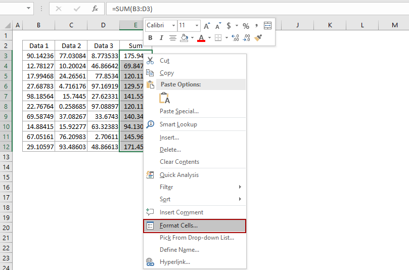
1. Pilih sel yang ingin Anda batasi jumlah tempat desimalnya.
2. Klik kanan sel yang dipilih, dan pilih Format Cells dari menu klik kanan.
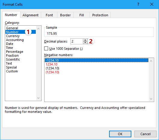
3. Di kotak dialog Format Sel yang akan datang, masuk ke Jumlah tab, klik untuk menyorot Jumlah dalam Kategori kotak, lalu ketikkan angka di Tempat desimal kotak.
Misalnya, jika Anda ingin membatasi hanya 1 tempat desimal untuk sel yang dipilih, ketik saja 1 ke dalam Tempat desimal kotak. Lihat tangkapan layar di bawah ini:
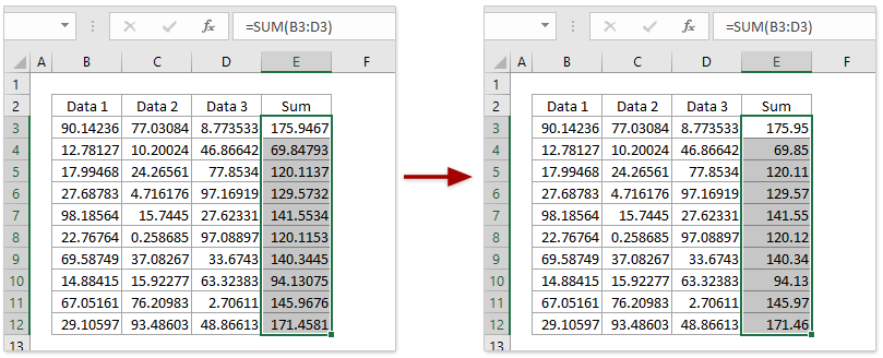
4. klik OK di kotak dialog Format Sel. Kemudian Anda akan melihat semua desimal di sel yang dipilih diubah menjadi satu tempat desimal.
Catatan: Setelah memilih sel, Anda dapat mengklik Tingkatkan Desimal tombol ![]() or Kurangi Desimal tombol
or Kurangi Desimal tombol ![]() langsung di Jumlah kelompok di Beranda tab untuk mengubah tempat desimal.
langsung di Jumlah kelompok di Beranda tab untuk mengubah tempat desimal.
Batasi dengan mudah jumlah tempat desimal dalam beberapa rumus di Excel
Secara umum, Anda dapat menggunakan = Round (original_formula, num_digits) untuk membatasi jumlah tempat desimal dalam satu rumus dengan mudah. Namun, akan sangat membosankan dan memakan waktu untuk mengubah beberapa rumus satu per satu secara manual. Di sini, gunakan fitur Operasi Kutools for Excel, Anda dapat dengan mudah membatasi jumlah tempat desimal dalam berbagai rumus dengan mudah!
Kutools untuk Excel - Tingkatkan Excel dengan lebih dari 300 alat penting. Nikmati uji coba GRATIS 30 hari berfitur lengkap tanpa memerlukan kartu kredit! Get It Now
Batasi jumlah tempat desimal dalam rumus di Excel
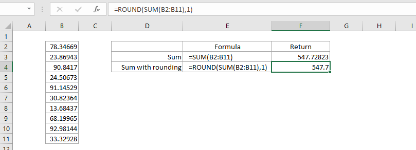
Katakanlah Anda menghitung jumlah rangkaian angka, dan Anda ingin membatasi jumlah tempat desimal untuk nilai penjumlahan ini dalam rumus, bagaimana Anda bisa menyelesaikannya di Excel? Anda harus mencoba fungsi Round.
Sintaks rumus Putaran dasar adalah:
= ROUND (angka, num_digits)
Dan jika Anda ingin menggabungkan fungsi Round dan rumus lainnya, sintaks rumus harus diubah menjadi
= Bulat (original_formula, num_digits)
Dalam kasus kami, kami ingin membatasi satu tempat desimal untuk nilai penjumlahan, sehingga kami dapat menerapkan rumus di bawah ini:
= PUTARAN (SUM (B2: B11), 1)
Batasi jumlah tempat desimal dalam beberapa rumus secara massal
Jika Anda memiliki Kutools untuk Excel diinstal, Anda dapat menerapkannya Operasi fitur untuk mengubah beberapa rumus yang dimasukkan secara massal, seperti mengatur pembulatan di Excel. Harap lakukan sebagai berikut:
Kutools untuk Excel- Termasuk lebih dari 300 alat praktis untuk Excel. Uji coba gratis fitur lengkap 30 hari, tidak perlu kartu kredit! Get It Now
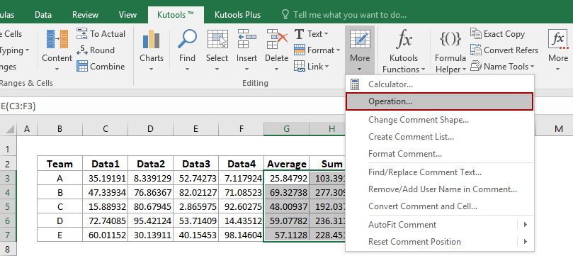
1. Pilih sel rumus yang tempat desimalnya perlu Anda batasi, dan klik Kutools > More > Operasi.
2. Dalam dialog Alat Operasi, klik untuk menyorot pembulatan dalam Operasi kotak daftar, ketik jumlah tempat desimal di Operan bagian, dan periksa Buat rumus .
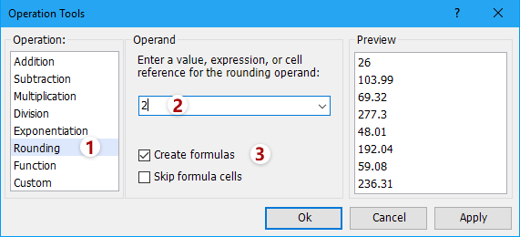
3. klik Ok .
Sekarang Anda akan melihat semua sel formula dibulatkan ke tempat desimal yang ditentukan secara massal. Lihat tangkapan layar:
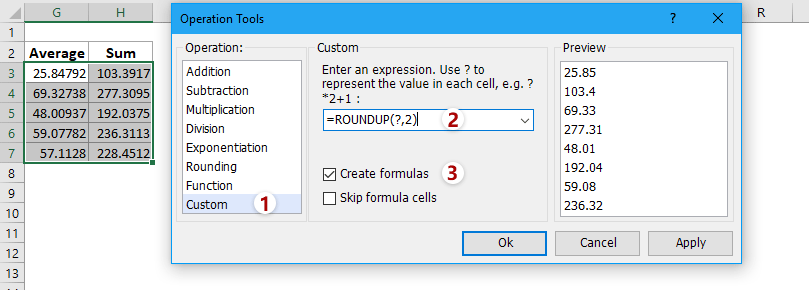
jenis: Jika Anda perlu membulatkan ke bawah atau mengumpulkan beberapa sel rumus secara massal, Anda dapat menyetel sebagai berikut: dalam dialog Alat Operasi, (1) memilih Kustom di kotak daftar Operasi, (2) mengetik = ROUNDUP (?, 2) or = ROUNDDOWN (?, 2) dalam Kustom bagian, dan (3) Periksalah Buat rumus pilihan. Lihat tangkapan layar:
Batasi dengan mudah jumlah tempat desimal dalam beberapa rumus di Excel
Biasanya fitur Desimal dapat mengurangi tempat desimal dalam sel, tetapi nilai aktual yang ditampilkan di bilah rumus tidak berubah sama sekali. Kutools untuk Excel'S bulat utilitas dapat membantu Anda membulatkan nilai ke atas / bawah / bahkan ke tempat desimal yang ditentukan dengan mudah.
Kutools untuk Excel- Termasuk lebih dari 300 alat praktis untuk Excel. Uji coba gratis fitur lengkap 60 hari, tidak perlu kartu kredit! Get It Now
Metode ini akan membulatkan sel rumus ke jumlah tempat desimal tertentu secara massal. Namun, ini akan menghapus rumus dari sel rumus ini dan hanya menyisakan hasil pembulatan.
Demo: batasi jumlah tempat desimal dalam rumus di Excel
Artikel terkait:
Alat Produktivitas Kantor Terbaik
Tingkatkan Keterampilan Excel Anda dengan Kutools for Excel, dan Rasakan Efisiensi yang Belum Pernah Ada Sebelumnya. Kutools for Excel Menawarkan Lebih dari 300 Fitur Lanjutan untuk Meningkatkan Produktivitas dan Menghemat Waktu. Klik Di Sini untuk Mendapatkan Fitur yang Paling Anda Butuhkan...
")
Tab Office Membawa antarmuka Tab ke Office, dan Membuat Pekerjaan Anda Jauh Lebih Mudah
- Aktifkan pengeditan dan pembacaan tab di Word, Excel, PowerPoint, Publisher, Access, Visio, dan Project.
- Buka dan buat banyak dokumen di tab baru di jendela yang sama, bukan di jendela baru.
- Meningkatkan produktivitas Anda sebesar 50%, dan mengurangi ratusan klik mouse untuk Anda setiap hari!
")