Loncat ke daftar isi utama

Bagaimana cara VLOOKUP dan mengembalikan beberapa nilai yang sesuai secara horizontal di Excel?

Penulis: Matahari Terakhir Dimodifikasi: 2020-04-22
doc-vlookup-horizontal-1
Secara default, fungsi VLOOKUP dapat mengembalikan beberapa nilai yang sesuai di tingkat vertikal di Excel, dalam beberapa kasus, Anda mungkin ingin mengembalikan beberapa nilai di tingkat horizontal seperti gambar di bawah ini. Di sini saya akan memberi tahu Anda rumus yang dapat menyelesaikan tugas ini.
VLOOKUP dan kembalikan beberapa nilai secara horizontal

panah gelembung kanan biru VLOOKUP dan kembalikan beberapa nilai secara horizontal

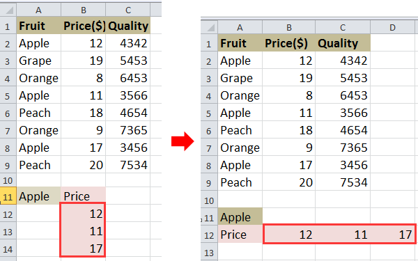
Misalnya, Anda memiliki berbagai data seperti gambar di bawah ini yang ditampilkan, dan Anda ingin VLOOKUP harga Apple.
doc-vlookup-horizontal-2

1. Pilih sel dan ketikkan rumus ini =INDEX($B$2:$B$9, SMALL(IF($A$11=$A$2:$A$9, ROW($A$2:$A$9)-ROW($A$2)+1), COLUMN(A1))) ke dalamnya, lalu tekan Shift + Ctrl + Masuk dan seret tuas IsiOtomatis ke kanan untuk menerapkan rumus ini hingga #JUMLAH! muncul. Lihat tangkapan layar:
doc-vlookup-horizontal-3

2. Kemudian hapus #NUM !. Lihat tangkapan layar:
doc-vlookup-horizontal-4

olymp trade indonesiaTip: Dalam rumus di atas, B2: B9 adalah rentang kolom yang ingin Anda kembalikan nilainya, A2: A9 adalah rentang kolom tempat nilai pencarian berada, A11 adalah nilai pencarian, A1 adalah sel pertama dari rentang data Anda , A2 adalah sel pertama dari rentang kolom tempat Anda mencari nilai.

Jika Anda ingin mengembalikan beberapa nilai secara vertikal, Anda dapat membaca artikel ini Bagaimana cara mencari nilai mengembalikan beberapa nilai yang sesuai di Excel?


Gabungkan beberapa lembar / Buku Kerja dengan mudah menjadi satu lembar atau Buku Kerja

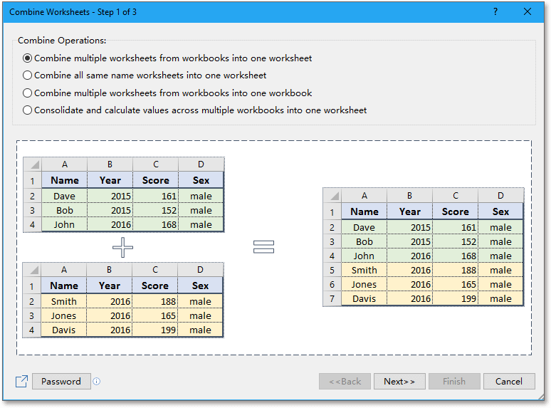
Untuk menggabungkan beberapa lembar atau buku kerja ke dalam satu lembar atau buku kerja mungkin membosankan di Excel, tapi dengan Menggabungkan Fungsi di Kutools for Excel, Anda bisa menggabungkan lusinan lembar / buku kerja menjadi satu lembar atau buku kerja, juga, Anda bisa menggabungkan lembaran menjadi satu dengan beberapa klik saja.  Klik untuk uji coba gratis 30 hari berfitur lengkap!
menggabungkan lembaran
 
Kutools for Excel: dengan lebih dari 300 add-in Excel yang praktis, gratis untuk dicoba tanpa batasan dalam 30 hari.

Alat Produktivitas Kantor Terbaik

馃 Kutools AI Ajudan: Merevolusi analisis data berdasarkan: Eksekusi Cerdas   |  Hasilkan Kode  |  Buat Rumus Khusus  |  Analisis Data dan Hasilkan Grafik  |  Aktifkan Fungsi Kutools...
Fitur Populer: Temukan, Sorot, atau Identifikasi Duplikat   |  Hapus Baris Kosong   |  Gabungkan Kolom atau Sel tanpa Kehilangan Data   |   Putaran tanpa Formula ...
Pencarian Super: VLookup Beberapa Kriteria    VLookup Nilai Berganda  |   VLookup di Beberapa Lembar   |   Pencarian Fuzzy ....
Daftar Drop-down Lanjutan: Buat Daftar Drop Down dengan Cepat   |  Daftar Drop Down yang Bergantung   |  Multi-pilih Drop Down List ....
Manajer Kolom: Tambahkan Jumlah Kolom Tertentu  |  Pindahkan Kolom  |  Alihkan Status Visibilitas Kolom Tersembunyi  |  Bandingkan Rentang & Kolom ...
Fitur Unggulan: Fokus Kisi   |  Tampilan Desain   |   Bar Formula Besar    Manajer Buku Kerja & Lembar   |  Perpustakaan Sumberdaya (Teks otomatis)   |  Pemetik tanggal   |  Gabungkan Lembar Kerja   |  Enkripsi/Dekripsi Sel    Kirim Email berdasarkan Daftar   |  Filter Super   |   Filter Khusus (filter tebal/miring/coret...) ...
15 Perangkat Teratas12 Teks Tools (Tambahkan Teks, Hapus Karakter, ...)   |   50 + Grafik jenis (Gantt Chart, ...)   |   40+ Praktis Rumus (Hitung usia berdasarkan ulang tahun, ...)   |   19 Insersi Tools (Masukkan Kode QR, Sisipkan Gambar dari Jalur, ...)   |   12 Konversi Tools (Angka ke Kata, Konversi Mata Uang, ...)   |   7 Gabungkan & Pisahkan Tools (Lanjutan Gabungkan Baris, Pisahkan Sel, ...)   |   ... dan banyak lagi

Tingkatkan Keterampilan Excel Anda dengan Kutools for Excel, dan Rasakan Efisiensi yang Belum Pernah Ada Sebelumnya. Kutools for Excel Menawarkan Lebih dari 300 Fitur Lanjutan untuk Meningkatkan Produktivitas dan Menghemat Waktu.  Klik Di Sini untuk Mendapatkan Fitur yang Paling Anda Butuhkan...

Deskripsi Produk


Tab Office Membawa antarmuka Tab ke Office, dan Membuat Pekerjaan Anda Jauh Lebih Mudah

  • Aktifkan pengeditan dan pembacaan tab di Word, Excel, PowerPoint, Publisher, Access, Visio, dan Project.
  • Buka dan buat banyak dokumen di tab baru di jendela yang sama, bukan di jendela baru.
  • Meningkatkan produktivitas Anda sebesar 50%, dan mengurangi ratusan klik mouse untuk Anda setiap hari!
Comments (20)
No ratings yet. Be the first to rate!
This comment was minimized by the moderator on the site
This article says this uses VLOOKUP, but it uses INDEX... which does not help me. I need a solution for multiple values using VLOOKUP or XLOOKUP in tables.
This comment was minimized by the moderator on the site
you can use TEXTSPLIT function followed by TEXTJOIN FUNCTION in excel 365
This comment was minimized by the moderator on the site
For anyone experiencing issues in a big data range, ensure you dont have any cells existent with "#N/A" or it will break it. Simple error but can be overlooked.
This comment was minimized by the moderator on the site
Hello, I want to use keyword instead of specific text or value here for multiple return values, can you please share code formula for same.
This comment was minimized by the moderator on the site
Hello - This formula worked perfectly - thank you! However, I want to apply it to a long list of lookup values. When I copy and paste the formula it obviously returns the same results as the first lookup value so I removed the $'s from $A$11, but that changes the result to something incorrect. How can I quickly apply this same formula for a long list of lookup values?

Thank you!

M
This comment was minimized by the moderator on the site
Bonjour,

J'ai retranspos茅 mon probl猫me exactement dans les m锚mes positions de colonne que l'exemple et j鈥檕btiens le message #VALEUR! d猫s la premi猫re case.

Mon excel fonctionne en francais, j'ai tout retranscrit en francais, pass茅 ";"au lieu de ",", appuy茅 sur CTRL+MAJ+Entr茅e... des id茅es sur l'origine du probl猫me?

Fanny
This comment was minimized by the moderator on the site
what you want to put the price in order of highest qty from column c?
This comment was minimized by the moderator on the site
i have to find vertical value first, in vertical value there are more horizontal value and i have choose grater value which i have. which function or formula can help
This comment was minimized by the moderator on the site
Hi. I have three google spreadsheet. First sheet is named "Summary. It is a table containing the name of our employee and number of evaluation in a week from 1-7. The next sheet is named "Chat Score"and third sheet is named 脣mail Score". What I want to to do is when we input a evaluation score to one of our employee it will be automatically recorded on the "Summary sheet" as evaluation 1 or 2 and so on and so forth. In short I want to get multiple return value in a single seach key across multiple sheet. I hope you can help. https://docs.google.com/spreadsheets/d/1lt-e4MxddUKg5xDt_0YchBiEgGe4mFKB-dHENwwtA6Y/edit?usp=sharing

https://docs.google.com/spreadsheets/d/1lt-e4MxddUKg5xDt_0YchBiEgGe4mFKB-dHENwwtA6Y/edit?usp=sharing
This comment was minimized by the moderator on the site
Although I'm looking up my values in another worksheet (I don't think this should cause a problem?), I only seem to have success dragging to the right if I go in and change the +1 to '0' for the 1st instance of the lookup ID, '1' for the 2nd instance and so on. I know how many instances of the lookup ID I have so I can workaround. What do I need to change to allow me to successfully drag the fx across horizontally without needing to edit (i.e getting the #NUM to appear once there are no more lookup values to return).
This comment was minimized by the moderator on the site
Sorry, I have not found any solutions about your problems. If you have found that, could you tell me? Thank u.
This comment was minimized by the moderator on the site
Change Column to Row at the end of the formula

"=INDEX($B$1:$B$206, SMALL(IF($A$209=$A$1:$A$206, ROW($A$1:$A$206)-ROW($A$1)+1), ROW(A1)))"
This comment was minimized by the moderator on the site
How to List all values(like list of groceries bought) caused by a specific value (by a person X) using VLOOK_UP and other possible formulas
This comment was minimized by the moderator on the site
You mean that to list all grocerise a person need to buy, right? If so, you can refer to the formula in this article, and change the arguments as you need as below screenshot shown.
There are no comments posted here yet
Load More
Please leave your comments in English
Posting as Guest
Rate this post:
0   Characters
Suggested Locations