Loncat ke daftar isi utama

Bagaimana cara membuat daftar drop-down dependen di lembar Google?

Memasukkan daftar drop-down normal di lembar Google mungkin merupakan pekerjaan yang mudah bagi Anda, tetapi, terkadang, Anda mungkin perlu memasukkan daftar drop-down dependen yang berarti daftar drop-down kedua tergantung pada pilihan daftar drop-down pertama. Bagaimana Anda bisa menangani tugas ini di lembar Google?

Buat daftar drop-down dependen di lembar Google


Buat daftar drop-down dependen di lembar Google

Langkah-langkah berikut dapat membantu Anda memasukkan daftar drop-down dependen, lakukan seperti ini:

1. Pertama, Anda harus memasukkan daftar drop-down dasar, pilih sel tempat Anda ingin meletakkan daftar drop-down pertama, lalu klik Data > Validasi data, lihat tangkapan layar:

2. Di muncul keluar Validasi data kotak dialog, pilih Daftar dari berbagai dari daftar tarik-turun di samping Kriteria bagian, lalu klik untuk memilih nilai sel yang ingin Anda buat berdasarkan daftar drop-down pertama, lihat tangkapan layar:

3. Lalu klik Save tombol, daftar drop-down pertama telah dibuat. Pilih satu item dari daftar drop-down yang dibuat, lalu masukkan rumus ini: =arrayformula(if(F1=A1,A2:A7,if(F1=B1,B2:B6,if(F1=C1,C2:C7,"")))) ke dalam sel kosong yang berdekatan dengan kolom data, lalu tekan Enter kunci, semua nilai yang cocok berdasarkan item daftar drop-down pertama telah ditampilkan sekaligus, lihat tangkapan layar:

Note: Dalam rumus di atas: F1 adalah sel daftar drop-down pertama, A1, B1 dan C1 adalah item dari daftar drop-down pertama, A2: A7, B2: B6 dan C2: C7 adalah nilai sel yang menjadi dasar daftar drop-down kedua. Anda dapat mengubahnya menjadi milik Anda.

4. Dan kemudian Anda dapat membuat daftar drop-down dependen kedua, klik sel tempat Anda ingin meletakkan daftar drop-down kedua, lalu klik Data > Validasi data untuk pergi ke Validasi data kotak dialog, pilih Daftar dari berbagai dari tarik-turun di samping Kriteria bagian, dan lanjutkan mengklik tombol untuk memilih sel formula yang merupakan hasil yang cocok dari item drop-down pertama, lihat tangkapan layar:

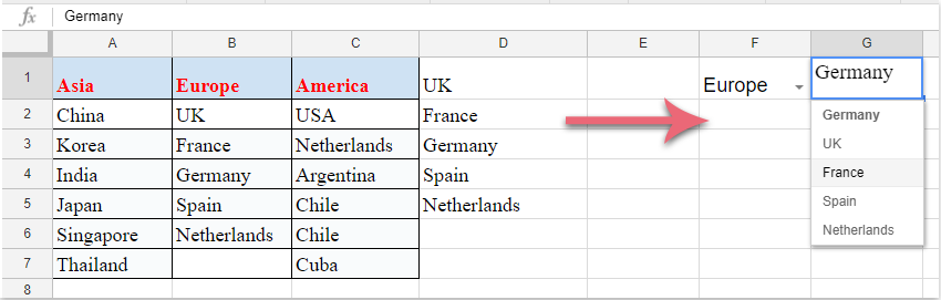
5. Terakhir, klik tombol Simpan, dan daftar drop-down dependen kedua telah berhasil dibuat seperti gambar berikut yang ditampilkan:

Alat Produktivitas Kantor Terbaik

🤖 Kutools AI Ajudan: Merevolusi analisis data berdasarkan: Eksekusi Cerdas   |  Hasilkan Kode  |  Buat Rumus Khusus  |  Analisis Data dan Hasilkan Grafik  |  Aktifkan Fungsi Kutools...
Fitur Populer: Temukan, Sorot, atau Identifikasi Duplikat   |  Hapus Baris Kosong   |  Gabungkan Kolom atau Sel tanpa Kehilangan Data   |   Putaran tanpa Formula ...
Pencarian Super: VLookup Beberapa Kriteria    VLookup Nilai Berganda  |   VLookup di Beberapa Lembar   |   Pencarian Fuzzy ....
Daftar Drop-down Lanjutan: Buat Daftar Drop Down dengan Cepat   |  Daftar Drop Down yang Bergantung   |  Multi-pilih Drop Down List ....
Manajer Kolom: Tambahkan Jumlah Kolom Tertentu  |  Pindahkan Kolom  |  Alihkan Status Visibilitas Kolom Tersembunyi  |  Bandingkan Rentang & Kolom ...
Fitur Unggulan: Fokus Kisi   |  Tampilan Desain   |   Bar Formula Besar    Manajer Buku Kerja & Lembar   |  Perpustakaan Sumberdaya (Teks otomatis)   |  Pemetik tanggal   |  Gabungkan Lembar Kerja   |  Enkripsi/Dekripsi Sel    Kirim Email berdasarkan Daftar   |  Filter Super   |   Filter Khusus (filter tebal/miring/coret...) ...
15 Perangkat Teratas12 Teks Tools (Tambahkan Teks, Hapus Karakter, ...)   |   50 + Grafik jenis (Gantt Chart, ...)   |   40+ Praktis Rumus (Hitung usia berdasarkan ulang tahun, ...)   |   19 Insersi Tools (Masukkan Kode QR, Sisipkan Gambar dari Jalur, ...)   |   12 Konversi Tools (Angka ke Kata, Konversi Mata Uang, ...)   |   7 Gabungkan & Pisahkan Tools (Lanjutan Gabungkan Baris, Pisahkan Sel, ...)   |   ... dan banyak lagi

Tingkatkan Keterampilan Excel Anda dengan Kutools for Excel, dan Rasakan Efisiensi yang Belum Pernah Ada Sebelumnya. Kutools for Excel Menawarkan Lebih dari 300 Fitur Lanjutan untuk Meningkatkan Produktivitas dan Menghemat Waktu.  Klik Di Sini untuk Mendapatkan Fitur yang Paling Anda Butuhkan...

Deskripsi Produk


Tab Office Membawa antarmuka Tab ke Office, dan Membuat Pekerjaan Anda Jauh Lebih Mudah

  • Aktifkan pengeditan dan pembacaan tab di Word, Excel, PowerPoint, Publisher, Access, Visio, dan Project.
  • Buka dan buat banyak dokumen di tab baru di jendela yang sama, bukan di jendela baru.
  • Meningkatkan produktivitas Anda sebesar 50%, dan mengurangi ratusan klik mouse untuk Anda setiap hari!
Comments (18)
No ratings yet. Be the first to rate!
This comment was minimized by the moderator on the site
Hi there. Its been working but for it only appears that only one cell can be formulated.I need help 
For example: in Cell A1, it shows dependent dropdown, but when in cell a2 it does not work.
Thas what help that i need, From A:A, They have all different selection from the dropdown list. Thanks.
This comment was minimized by the moderator on the site
Would it been possible to create pull down menu based of formula?
I use formula "=SUMIFS(Items!$I:$I,Items!$A:$A,K$1,Items!$D:$D,$D2)" (=for example 150) to find the qty on pallet based on item and container size.
So I wanted to create pull down menu like qty 1 pallet, qty 2 pallets, qty 3 pallets,.....
Then user will always order qty of full pallets like 150, 2 x 150, 3 x150, up to 21 x 150.
This comment was minimized by the moderator on the site
Hi, I already created a drop down list like this one, what I'd like to know is how i can, when clicking on one option from that list, restrict what appears as options on another cell. For example, in one cell i can choose between laparoscopy and orthopaedics. If I choose orthopaedics then, the other cell which has a list of doctors, should only show the doctors for orthopedy and not all of them. Does anyone know how to do this?
This comment was minimized by the moderator on the site
Hii Sir,
I Want to Create A Dependent Drop Down List Like
- State(A1):- District(B1):- Taluka(C1) :- Then Information(D1) ,
So I need your Help .
Tell How do you do this Type of Dependent Drop down List in Excel or Google Sheet
This comment was minimized by the moderator on the site
Hi, Shelate,
Maybe the below article can solve your problem, please view it:
https://www.extendoffice.com/documents/excel/5852-excel-multiple-level-drop-down-list.html

Please try, hope it can help you!
This comment was minimized by the moderator on the site
Now is needed to use: =arrayformula(if(F1=A1;A2:A7;if(F1=B1;B2:B6;if(F1=C1;C2:C7;""))))
This comment was minimized by the moderator on the site
Thank you soooo much!
This comment was minimized by the moderator on the site
Hi,
I was wondering if anyone could advise me with this? I've followed the above steps but on step 3 rather than getting:
"...all the matching values based on the first drop down list item have been displayed at once," I am just seeing one value (the top one from the drop down list).
My cells are placed slightly differently and the first drop down is filled from another sheet (from anywhere int eh column excluding the top row) so my formula is:

=arrayformula(if(VLE!D2:D=B11,B12,if(VLE!D2:D=C11,C12:C14,if(VLE!D2:D=D11,D12:D14,if(VLE!D2:D=E11,E12:E16,if(VLE!D2:D=F11,F12:F16,""))))))

It is correctly displaying the top drop down option for each of (using cell numbers from the step 3 example on this page) A1, B1, and C1 so, again using this page's example, if I select Asia form the F1 drop down, I would get China, but nothing further


Any suggestions?

Many thanks! Nick
This comment was minimized by the moderator on the site
If the first drop own is on sheet 1 A1, will this work were I want the second drop down as sheet 1 A2, but to have its data range on a separate sheet?
This comment was minimized by the moderator on the site
Ich bekomm immer die Meldung "Fehler beim Parsen der Formel" wenn ich =arrayformula(if(F1=A1,A2:A7,if(F1=B1,B2:B6,if(F1=C1,C2:C7,"")))) eingebe. Was ist der "Weiter-Schlüsel"? Reicht es nicht wie bei Excel die Formel einzugeben?
This comment was minimized by the moderator on the site
Ersetzen Sie den , zu ;
es hat für mich funktioniert
This comment was minimized by the moderator on the site
This is the best explanation I have found, so thank you for that!

In my situation, I am working with over 200 rows with more being continuously added. Is there an easier/more efficient way to handle this many rows?
This comment was minimized by the moderator on the site
Yes, if you don't put number index to specify ending cell.
Like instead of C2:C7 you put C2:C. This will automatically tell the array formula, that you want to consider all values in column "C" starting at "C2".
This comment was minimized by the moderator on the site
What happens if I want exactly the same dropdown list in F2 as you have in F1 ?
I tried, and it doesn't overwrite D1:D7 .. meaning D1:D7 is only available once.
I need something else, double dropdown, but on many-many lines .. guess I must use another system then .. not sure which ..
This comment was minimized by the moderator on the site
Hi, Xained,
This method can only applied to one cell, if you have some good ways for applying this to multiple cells, please comment here.

Thank you!
This comment was minimized by the moderator on the site
Please, guide me how to do that.Thanks
This comment was minimized by the moderator on the site
혹시, 하나의 셀이 아닌 여러셀에 할 수 있는 방법을 알 수 있을까요?
This comment was minimized by the moderator on the site
내말이... 시바 좃빠지게 따라했디만 밑에줄은 안되노..
There are no comments posted here yet
Please leave your comments in English
Posting as Guest
×
Rate this post:
0   Characters
Suggested Locations