Loncat ke daftar isi utama

Bagaimana cara menyembunyikan sebagian dari nilai sel di Excel?

Penulis: Matahari Terakhir Dimodifikasi: 2020-05-27
doc sembunyikan sebagian 1
Misalkan Anda memiliki lembar dengan beberapa informasi umum tentang staf, tetapi beberapa bersifat pribadi seperti nomor jaminan sosial. Sekarang Anda ingin menyembunyikan bagian dari nomor jaminan sosial ini seperti gambar di bawah ini, bagaimana Anda bisa menyelesaikannya dengan cepat?

Sembunyikan sebagian nomor jaminan sosial dengan Format Cells

Sembunyikan sebagian teks atau angka dengan rumus

panah gelembung kanan biru Sembunyikan sebagian nomor jaminan sosial dengan Format Cells

Untuk menyembunyikan bagian dari nomor jaminan sosial di Excel, Anda bisa menerapkan Format Cells untuk mengatasinya.

1. Pilih nomor yang ingin Anda sembunyikan sebagian, dan klik kanan untuk memilih Format Cells dari menu konteks. Lihat tangkapan layar:
doc sembunyikan sebagian 2

2. Kemudian di Format Cells dialog, klik Jumlah tab, dan pilih Kustom dari Kategori panel, dan pergi untuk memasukkan ini 000 ,, "- ** - ****" ke dalam Tipe kotak di bagian kanan. Lihat tangkapan layar:
doc sembunyikan sebagian 3

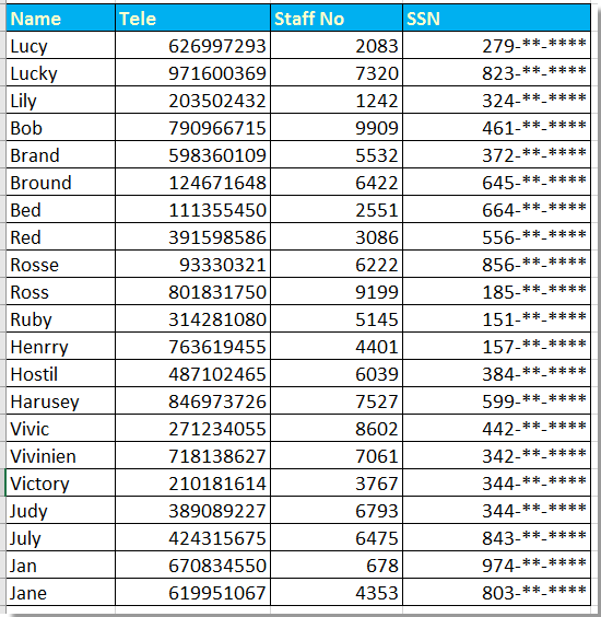
3. klik OK, sekarang sebagian nomor yang Anda pilih telah disembunyikan.

Note: Akan membulatkan angka jika angka keempat lebih besar dari atau eaqul menjadi 5.


panah gelembung kanan biru Sembunyikan sebagian teks atau angka dengan rumus

Dengan metode di atas, Anda hanya dapat menyembunyikan nomor parsial, jika Anda ingin menyembunyikan sebagian atau teks, Anda dapat melakukan seperti di bawah ini:

Di sini kami menyembunyikan 4 nomor pertama dari nomor paspor.

Pilih satu sel kosong di sebelah nomor paspor, F22 misalnya, masukkan rumus ini = "****" & KANAN (E22,5), lalu seret gagang IsiOtomatis ke sel yang Anda perlukan untuk menerapkan rumus ini.
doc sembunyikan sebagian 4

olymp trade indonesiaTip:

Jika Anda ingin menyembunyikan empat angka terakhir, gunakan rumus ini, = KIRI (H2,5) & "****"

Jika Anda ingin menyembunyikan tiga angka tengah, gunakan ini = KIRI (H2,3) & "***" & KANAN (H2,3)

Alat Produktivitas Kantor Terbaik

🤖 Kutools AI Ajudan: Merevolusi analisis data berdasarkan: Eksekusi Cerdas   |  Hasilkan Kode  |  Buat Rumus Khusus  |  Analisis Data dan Hasilkan Grafik  |  Aktifkan Fungsi Kutools...
Fitur Populer: Temukan, Sorot, atau Identifikasi Duplikat   |  Hapus Baris Kosong   |  Gabungkan Kolom atau Sel tanpa Kehilangan Data   |   Putaran tanpa Formula ...
Pencarian Super: VLookup Beberapa Kriteria    VLookup Nilai Berganda  |   VLookup di Beberapa Lembar   |   Pencarian Fuzzy ....
Daftar Drop-down Lanjutan: Buat Daftar Drop Down dengan Cepat   |  Daftar Drop Down yang Bergantung   |  Multi-pilih Drop Down List ....
Manajer Kolom: Tambahkan Jumlah Kolom Tertentu  |  Pindahkan Kolom  |  Alihkan Status Visibilitas Kolom Tersembunyi  |  Bandingkan Rentang & Kolom ...
Fitur Unggulan: Fokus Kisi   |  Tampilan Desain   |   Bar Formula Besar    Manajer Buku Kerja & Lembar   |  Perpustakaan Sumberdaya (Teks otomatis)   |  Pemetik tanggal   |  Gabungkan Lembar Kerja   |  Enkripsi/Dekripsi Sel    Kirim Email berdasarkan Daftar   |  Filter Super   |   Filter Khusus (filter tebal/miring/coret...) ...
15 Perangkat Teratas12 Teks Tools (Tambahkan Teks, Hapus Karakter, ...)   |   50 + Grafik jenis (Gantt Chart, ...)   |   40+ Praktis Rumus (Hitung usia berdasarkan ulang tahun, ...)   |   19 Insersi Tools (Masukkan Kode QR, Sisipkan Gambar dari Jalur, ...)   |   12 Konversi Tools (Angka ke Kata, Konversi Mata Uang, ...)   |   7 Gabungkan & Pisahkan Tools (Lanjutan Gabungkan Baris, Pisahkan Sel, ...)   |   ... dan banyak lagi

Tingkatkan Keterampilan Excel Anda dengan Kutools for Excel, dan Rasakan Efisiensi yang Belum Pernah Ada Sebelumnya. Kutools for Excel Menawarkan Lebih dari 300 Fitur Lanjutan untuk Meningkatkan Produktivitas dan Menghemat Waktu.  Klik Di Sini untuk Mendapatkan Fitur yang Paling Anda Butuhkan...

Deskripsi Produk


Tab Office Membawa antarmuka Tab ke Office, dan Membuat Pekerjaan Anda Jauh Lebih Mudah

  • Aktifkan pengeditan dan pembacaan tab di Word, Excel, PowerPoint, Publisher, Access, Visio, dan Project.
  • Buka dan buat banyak dokumen di tab baru di jendela yang sama, bukan di jendela baru.
  • Meningkatkan produktivitas Anda sebesar 50%, dan mengurangi ratusan klik mouse untuk Anda setiap hari!
Comments (21)
No ratings yet. Be the first to rate!
This comment was minimized by the moderator on the site
I have 1. Name, so I want to remove "1." Please suggest.
This comment was minimized by the moderator on the site
Is there any command for format cell, to hide the intended value in cell, that containt with charecters. eg. G1234567Q and after applied the format it would be G****567Q ?Note: I am asking to know the cell format not the formula? Thanks in advance!
This comment was minimized by the moderator on the site
If I have a listing of Name with different length, and want to set as "B*** P***" for "Brad Pitt", "M******* Y*** C*** K****" for "Michelle Yeoh Choo Kheng", how can I do it with formula?
p     JL
This comment was minimized by the moderator on the site
have you found a solution? i would also like to know the answer to this. thank you
This comment was minimized by the moderator on the site
Can replace all but the first char with this: =REPLACE(CELL,2,LEN(CELL),REPT("*",LEN(CELL)))
This comment was minimized by the moderator on the site
If I have a number and alphabet set like S1234567A and want to put as S****567A, what formula is usable?
This comment was minimized by the moderator on the site
=REPLACE(CELL,2,4,"****")
This comment was minimized by the moderator on the site
=REPLACE(CELL,1,LEN(CELL)-4,REPT("X",LEN(CELL)-4))is the better version as here you can mask text with variable length
This comment was minimized by the moderator on the site
Hi I tried this but does not seem to work.
This comment was minimized by the moderator on the site
Great solution!
This comment was minimized by the moderator on the site
How can we use format cell to remove the first few characters? For ex: 12,345.67 = **,345.67
This comment was minimized by the moderator on the site
how can i unhide the numbers again
This comment was minimized by the moderator on the site
Hi, sunil, if you use the Format Cells function to hide part of string, when you want to unhide them again, just format the cells as general.
This comment was minimized by the moderator on the site
Nice Sir, Its working
This comment was minimized by the moderator on the site
Sorry, I meant D22
This comment was minimized by the moderator on the site
I am not sure how you wrote the formula Dean, but =LEFT(F22,3)&"-**-****" shows 278-**-**** for me... Maybe check other formats on your destination cell?
This comment was minimized by the moderator on the site
Sorry I did not get your question, could you give me a screenshot or other more information to decribe it?
This comment was minimized by the moderator on the site
Your SSN example fails, in that it rounds up the number, rather than hiding the non-visible placings. In you example, 278-53-6128 is displayed as 279-**-****!
This comment was minimized by the moderator on the site
Sorry, could you give me more information about the fails in your examples? Because it works always in my examples.
This comment was minimized by the moderator on the site
Dean is correct, the image you are using for the example shows staff no 2083 having the social security number of 278536128 but the hidden version starts with 279. The formula itself works, just the first row in the example image is incorrect.
This comment was minimized by the moderator on the site
Thanks for the reminder. The format cell method will round up the number if the fourth number is larger than 5.
There are no comments posted here yet
Please leave your comments in English
Posting as Guest
×
Rate this post:
0   Characters
Suggested Locations