Bagaimana cara menggabungkan sel jika nilai yang sama ada di kolom lain di Excel?

Seperti yang ditunjukkan pada tangkapan layar di bawah ini, jika Anda ingin menggabungkan sel di kolom kedua berdasarkan nilai yang sama di kolom pertama, ada beberapa metode yang dapat Anda gunakan. Pada artikel ini, kami akan memperkenalkan tiga cara untuk menyelesaikan tugas ini.

Gabungkan sel jika nilainya sama dengan rumus dan filter

Rumus berikut membantu menggabungkan konten sel yang sesuai di kolom berdasarkan nilai yang sama di kolom lain.

1. Pilih sel kosong di samping kolom kedua (di sini kita pilih sel C2), masukkan rumus = IF (A2 <> A1, B2, C1 & "," & B2) ke dalam bilah rumus, lalu tekan Enter kunci.

2. Kemudian pilih sel C2, dan seret Fill Handle ke bawah ke sel yang perlu Anda gabungkan.

3. Masukkan rumus = IF (A2 <> A3, CONCATENATE (A2, "," "", C2, "" ""), "") ke dalam sel D2, dan seret Fill Handle ke sel lainnya.

4. Pilih sel D1, dan klik Data > Filter. Lihat tangkapan layar:

5. Klik panah drop-down di sel D1, hapus centang (Kosong) kotak, dan kemudian klik OK .

Anda dapat melihat sel-sel tersebut digabungkan jika nilai kolom pertama sama.

Note: Untuk menggunakan rumus di atas dengan sukses, nilai yang sama di kolom A harus kontinu.

Gabungkan sel dengan mudah jika nilainya sama dengan Kutools for Excel (beberapa klik)

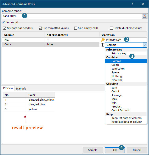
Metode yang dijelaskan di atas memerlukan pembuatan dua kolom pembantu dan melibatkan beberapa langkah, yang mungkin merepotkan. Jika Anda mencari cara yang lebih sederhana, pertimbangkan untuk menggunakan Lanjutan Gabungkan Baris alat dari Kutools untuk Excel. Hanya dengan beberapa klik, utilitas ini memungkinkan Anda menggabungkan sel menggunakan pembatas tertentu, menjadikan prosesnya cepat dan tidak merepotkan.

jenis: Sebelum menerapkan alat ini, harap instal Kutools untuk Excel pertama. Buka unduhan gratis sekarang.

• Pilih rentang yang ingin Anda gabungkan;
• Atur kolom dengan nilai yang sama dengan Kunci utama kolom.
• Tentukan pemisah untuk menggabungkan sel.
• Klik OK.

Hasil

Gabungkan sel jika nilainya sama dengan kode VBA

Anda juga dapat menggunakan kode VBA untuk menggabungkan sel dalam kolom jika nilai yang sama ada di kolom lain.

1. tekan lain + F11 kunci untuk membuka Aplikasi Microsoft Visual Basic jendela.

2. Dalam Aplikasi Microsoft Visual Basic window, klik Menyisipkan > Modul. Kemudian salin dan tempel kode di bawah ini ke dalam Modul jendela.

Kode VBA: menggabungkan sel jika nilainya sama

Sub ConcatenateCellsIfSameValues()
	Dim xCol As New Collection
	Dim xSrc As Variant
	Dim xRes() As Variant
	Dim I As Long
	Dim J As Long
	Dim xRg As Range
	xSrc    = Range("A1", Cells(Rows.Count, "A").End(xlUp)).Resize(, 2)
	Set xRg = Range("D1")
	On Error Resume Next
	For I = 2 To UBound(xSrc)
		xCol.Add xSrc(I, 1), TypeName(xSrc(I, 1)) & CStr(xSrc(I, 1))
	Next I
	On Error GoTo 0
	ReDim xRes(1 To xCol.Count + 1, 1 To 2)
	xRes(1, 1) = "No"
	xRes(1, 2) = "Combined Color"
	For I = 1 To xCol.Count
		xRes(I + 1, 1) = xCol(I)
		For J = 2 To UBound(xSrc)
			If xSrc(J, 1) = xRes(I + 1, 1) Then
				xRes(I + 1, 2) = xRes(I + 1, 2) & ", " & xSrc(J, 2)
			End If
		Next J
		xRes(I + 1, 2) = Mid(xRes(I + 1, 2), 2)
	Next I
	Set xRg = xRg.Resize(UBound(xRes, 1), UBound(xRes, 2))
	xRg.NumberFormat = "@"
	xRg = xRes
	xRg.EntireColumn.AutoFit
End Sub

Catatan:

3. tekan F5 kunci untuk menjalankan kode, maka Anda akan mendapatkan hasil gabungan dalam rentang yang ditentukan.

Gabungkan sel dengan mudah jika nilainya sama dengan Kutools for Excel

Alat Produktivitas Kantor Terbaik

🤖	Kutools AI Ajudan: Merevolusi analisis data berdasarkan: Eksekusi Cerdas   |  Hasilkan Kode  |  Buat Rumus Khusus  |  Analisis Data dan Hasilkan Grafik  |  Aktifkan Fungsi Kutools...
	Fitur Populer: Temukan, Sorot, atau Identifikasi Duplikat   |  Hapus Baris Kosong   |  Gabungkan Kolom atau Sel tanpa Kehilangan Data   |   Putaran tanpa Formula ...
	Pencarian Super: VLookup Beberapa Kriteria  |   VLookup Nilai Berganda  |   VLookup di Beberapa Lembar   |   Pencarian Fuzzy ....
	Daftar Drop-down Lanjutan: Buat Daftar Drop Down dengan Cepat   |  Daftar Drop Down yang Bergantung   |  Multi-pilih Drop Down List ....
	Manajer Kolom: Tambahkan Jumlah Kolom Tertentu  |  Pindahkan Kolom  |  Alihkan Status Visibilitas Kolom Tersembunyi  |  Bandingkan Rentang & Kolom ...
	Fitur Unggulan: Fokus Kisi   |  Tampilan Desain   |   Bar Formula Besar   |  Manajer Buku Kerja & Lembar   |  Perpustakaan Sumberdaya (Teks otomatis)   |  Pemetik tanggal   |  Gabungkan Lembar Kerja   |  Enkripsi/Dekripsi Sel   |  Kirim Email berdasarkan Daftar   |  Filter Super   |   Filter Khusus (filter tebal/miring/coret...) ...
	15 Perangkat Teratas:  12 Teks Tools (Tambahkan Teks, Hapus Karakter, ...)   |   50 + Grafik jenis (Gantt Chart, ...)   |   40+ Praktis Rumus (Hitung usia berdasarkan ulang tahun, ...)   |   19 Insersi Tools (Masukkan Kode QR, Sisipkan Gambar dari Jalur, ...)   |   12 Konversi Tools (Angka ke Kata, Konversi Mata Uang, ...)   |   7 Gabungkan & Pisahkan Tools (Lanjutan Gabungkan Baris, Pisahkan Sel, ...)   |   ... dan banyak lagi

Tingkatkan Keterampilan Excel Anda dengan Kutools for Excel, dan Rasakan Efisiensi yang Belum Pernah Ada Sebelumnya. Kutools for Excel Menawarkan Lebih dari 300 Fitur Lanjutan untuk Meningkatkan Produktivitas dan Menghemat Waktu.  Klik Di Sini untuk Mendapatkan Fitur yang Paling Anda Butuhkan...

Read More ... Download Gratis...

---

Tab Office Membawa antarmuka Tab ke Office, dan Membuat Pekerjaan Anda Jauh Lebih Mudah

• Aktifkan pengeditan dan pembacaan tab di Word, Excel, PowerPoint, Publisher, Access, Visio, dan Project.
• Buka dan buat banyak dokumen di tab baru di jendela yang sama, bukan di jendela baru.
• Meningkatkan produktivitas Anda sebesar 50%, dan mengurangi ratusan klik mouse untuk Anda setiap hari!

Read More ... Download Gratis...