Bagaimana cara membalikkan tanda nilai dalam sel di Excel?
Saat kami menggunakan excel, ada angka positif dan negatif di lembar kerja. Misalkan kita perlu mengubah angka positif menjadi negatif dan sebaliknya. Tentu kita bisa mengubahnya secara manual, tapi jika ada ratusan nomor yang perlu diubah, cara ini bukan pilihan yang baik. Apakah ada trik cepat untuk mengatasi masalah ini?
 |
 |
 |
Membalikkan tanda nilai dalam sel dengan fungsi Tempel Spesial
Balikkan tanda nilai dalam sel dengan Kutools for Excel dengan cepat
Membalikkan tanda nilai dalam sel dengan fungsi Tempel Spesial

Kita bisa membalikkan tanda nilai dalam sel dengan sisipkan Khusus fungsi di Excel, lakukan hal berikut:
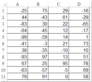
1. Ketuk nomor -1 di sel kosong dan salin.
2. Pilih rentang yang Anda ingin membalikkan tanda nilainya, klik kanan dan pilih sisipkan Khusus. Lihat tangkapan layar:

3. Dalam majalah sisipkan Khusus kotak dialog, klik Semua opsi dari pasta dan Mengalikan opsi dari Operasi. Lihat tangkapan layar:

4. Lalu klik OK, dan semua tanda angka dalam kisaran tersebut telah dibalik.
|
|
|
5. Hapus angka -1 sesuai kebutuhan.
Balikkan tanda semua angka sekaligus
Kutools untuk Excel'S Ubah Tanda Nilai utilitas dapat membantu Anda mengubah bilangan positif menjadi negatif dan sebaliknya, ini juga dapat membantu Anda membalikkan tanda nilai dan memperbaiki tanda negatif yang tertinggal menjadi normal. Klik untuk mengunduh Kutools for Excel!

Kutools untuk Excel: dengan lebih dari 300 add-in Excel yang praktis, gratis untuk dicoba tanpa batasan dalam 30 hari. Unduh dan uji coba gratis Sekarang!
Balikkan tanda nilai dalam sel dengan Kutools for Excel dengan cepat
Kita dapat membalikkan tanda nilai dengan cepat Ubah Tanda Nilai fitur dari Kutools untuk Excel.
| Kutools untuk Excel : dengan lebih dari 300 add-in Excel yang praktis, gratis untuk dicoba tanpa batasan dalam 30 hari. |
Setelah menginstal Kutools untuk Excel, lakukan hal berikut:
1. Pilih rentang yang Anda ingin membalikkan tanda-tanda angka.
2. Klik Kutools > Konten > Ubah Tanda Nilai…, Lihat tangkapan layar:

3. di Ubah Tanda Nilai kotak dialog, periksa Balikkan tanda semua nilai, lihat tangkapan layar:

4. Dan kemudian klik OK or Mendaftar. Semua tanda angka telah dibalik.
- Untuk menggunakan fitur ini, Anda harus menginstal Kutools untuk Excel pertama, silakan klik untuk mengunduh dan dapatkan uji coba gratis 30 hari sekarang.
- Grafik Ubah Tanda Nilai dari Kutools for Excel juga bisa perbaiki tanda-tanda negatif yang tertinggal, Cubah semua nilai negatif menjadi positif dan ubah semua nilai positif menjadi negatif. Untuk informasi lebih detail tentang Ubah Tanda Nilai, Silakan kunjungi Ubah deskripsi fitur Sign of Values.
Balikkan tanda nilai dalam sel dengan kode VBA
Juga, kita dapat menggunakan kode VBA untuk membalikkan tanda nilai dalam sel. Tapi kita harus tahu bagaimana membuat VBA melakukan hal itu. Kami dapat melakukannya sebagai langkah-langkah berikut:
1. Pilih rentang yang Anda inginkan untuk membalikkan tanda nilai dalam sel.
2. Klik Pengembang > Visual Basic di Excel, file Microsoft Visual Basic untuk aplikasi jendela akan ditampilkan, atau menggunakan tombol pintas (Alt + F11) untuk mengaktifkannya. Lalu klik Menyisipkan > Modul, lalu salin dan tempel kode VBA berikut ini:
Sub Convert()
Dim C As Range
For Each C In Selection
C.Value = -C.Value
Next C
End Sub
3. Kemudian klik ![]() tombol untuk menjalankan kode. Dan tanda angka dalam rentang yang dipilih telah dibalik sekaligus.
tombol untuk menjalankan kode. Dan tanda angka dalam rentang yang dipilih telah dibalik sekaligus.
Balikkan tanda nilai dalam sel dengan Kutools for Excel
Terkait artikel
Membalikkan tanda nilai dalam sel
Saat kami menggunakan excel, ada angka positif dan negatif di lembar kerja. Misalkan kita perlu mengubah angka positif menjadi negatif dan sebaliknya. Tentu kita bisa mengubahnya secara manual, tapi jika ada ratusan nomor yang perlu diubah, cara ini bukan pilihan yang baik. Apakah ada trik cepat untuk mengatasi masalah ini?
Ubah angka positif menjadi negatif
Bagaimana Anda bisa dengan cepat mengubah semua angka atau nilai positif menjadi negatif di Excel? Metode berikut dapat memandu Anda dengan cepat mengubah semua bilangan positif menjadi negatif di Excel.
Perbaiki tanda negatif yang tertinggal di sel
Untuk beberapa alasan, Anda mungkin perlu memperbaiki tanda negatif di sel di Excel. Misalnya, angka dengan tanda negatif di belakangnya akan menjadi seperti 90-. Dalam kondisi ini, bagaimana cara cepat memperbaiki trailing negative dengan menghilangkan trailing negative dari kanan ke kiri? Berikut beberapa trik cepat yang dapat membantu Anda.
Ubah angka negatif menjadi nol
Saya akan memandu Anda untuk mengubah semua angka negatif menjadi nol sekaligus dalam pilihan.
Alat Produktivitas Kantor Terbaik
Kutools for Excel - Membantu Anda Menonjol Dari Kerumunan
Kutools for Excel Membanggakan Lebih dari 300 Fitur, Memastikan Apa yang Anda Butuhkan Hanya Dengan Sekali Klik...
")
Tab Office - Aktifkan Pembacaan dan Pengeditan dengan Tab di Microsoft Office (termasuk Excel)
- Satu detik untuk beralih di antara lusinan dokumen terbuka!
- Kurangi ratusan klik mouse untuk Anda setiap hari, ucapkan selamat tinggal pada tangan mouse.
- Meningkatkan produktivitas Anda sebesar 50% saat melihat dan mengedit banyak dokumen.
- Menghadirkan Tab Efisien ke Office (termasuk Excel), Sama Seperti Chrome, Edge, dan Firefox.
")