Loncat ke daftar isi utama

Bagaimana rata-rata 5 nilai terakhir dari kolom saat angka baru masuk?

Pengarang: Xiaoyang Terakhir Dimodifikasi: 2020-07-24

Di Excel, Anda bisa dengan cepat menghitung rata-rata 5 nilai terakhir dalam kolom dengan fungsi Rata-rata, tetapi, dari waktu ke waktu, Anda perlu memasukkan angka baru di belakang data asli Anda, dan Anda ingin hasil rata-rata akan berubah secara otomatis sebagai data baru masuk. Artinya, Anda ingin rata-rata selalu mencerminkan 5 angka terakhir dari daftar data Anda, bahkan saat Anda menambahkan angka sesekali.

Rata-rata 5 nilai terakhir kolom sebagai angka baru yang dimasukkan dengan rumus


panah gelembung kanan biru Rata-rata 5 nilai terakhir kolom sebagai angka baru yang dimasukkan dengan rumus

Rumus array berikut dapat membantu Anda memecahkan masalah ini, lakukan hal berikut:

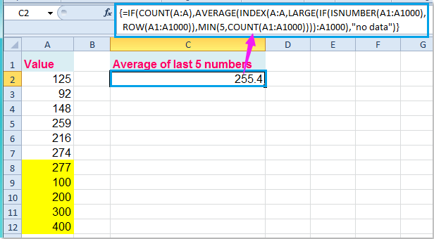
Masukkan rumus ini ke dalam sel kosong:

=IF(COUNT(A:A),AVERAGE(INDEX(A:A,LARGE(IF(ISNUMBER(A1:A10000),ROW(A1:A10000)),MIN(5,COUNT(A1:A10000)))):A10000),"no data") (A: A adalah kolom yang berisi data yang Anda gunakan, A1: A10000 adalah rentang dinamis, Anda dapat mengembangkannya selama kebutuhan Anda, dan jumlahnya 5 menunjukkan nilai n terakhir.), lalu tekan Ctrl + Shift + Enter kunci bersama untuk mendapatkan rata-rata dari 5 angka terakhir. Lihat tangkapan layar:

doc-rata-rata-terakhir-5-1

Dan sekarang, ketika Anda memasukkan angka baru di belakang data asli, rata-rata akan berubah juga, lihat tangkapan layar:

doc-rata-rata-terakhir-5-2

Note: Jika kolom sel berisi nilai 0, Anda ingin mengecualikan 0 nilai dari 5 angka terakhir Anda, rumus di atas tidak akan berfungsi, di sini, saya dapat memperkenalkan rumus array lain untuk mendapatkan rata-rata dari 5 nilai bukan nol terakhir , masukkan rumus ini:

=AVERAGE(SUBTOTAL(9,OFFSET(A1:A10000,LARGE(IF(A1:A10000>0,ROW(A1:A10000)-MIN(ROW(A1:A10000))),ROW(INDIRECT("1:5"))),0,1))), lalu tekan Ctrl + Shift + Enter kunci untuk mendapatkan hasil yang Anda butuhkan, lihat tangkapan layar:

doc-rata-rata-terakhir-5-3


Artikel terkait:

Bagaimana rata-rata setiap 5 baris atau kolom di Excel?

Bagaimana rata-rata nilai 3 atas atau bawah di Excel?

Alat Produktivitas Kantor Terbaik

馃 Kutools AI Ajudan: Merevolusi analisis data berdasarkan: Eksekusi Cerdas   |  Hasilkan Kode  |  Buat Rumus Khusus  |  Analisis Data dan Hasilkan Grafik  |  Aktifkan Fungsi Kutools...
Fitur Populer: Temukan, Sorot, atau Identifikasi Duplikat   |  Hapus Baris Kosong   |  Gabungkan Kolom atau Sel tanpa Kehilangan Data   |   Putaran tanpa Formula ...
Pencarian Super: VLookup Beberapa Kriteria    VLookup Nilai Berganda  |   VLookup di Beberapa Lembar   |   Pencarian Fuzzy ....
Daftar Drop-down Lanjutan: Buat Daftar Drop Down dengan Cepat   |  Daftar Drop Down yang Bergantung   |  Multi-pilih Drop Down List ....
Manajer Kolom: Tambahkan Jumlah Kolom Tertentu  |  Pindahkan Kolom  |  Alihkan Status Visibilitas Kolom Tersembunyi  |  Bandingkan Rentang & Kolom ...
Fitur Unggulan: Fokus Kisi   |  Tampilan Desain   |   Bar Formula Besar    Manajer Buku Kerja & Lembar   |  Perpustakaan Sumberdaya (Teks otomatis)   |  Pemetik tanggal   |  Gabungkan Lembar Kerja   |  Enkripsi/Dekripsi Sel    Kirim Email berdasarkan Daftar   |  Filter Super   |   Filter Khusus (filter tebal/miring/coret...) ...
15 Perangkat Teratas12 Teks Tools (Tambahkan Teks, Hapus Karakter, ...)   |   50 + Grafik jenis (Gantt Chart, ...)   |   40+ Praktis Rumus (Hitung usia berdasarkan ulang tahun, ...)   |   19 Insersi Tools (Masukkan Kode QR, Sisipkan Gambar dari Jalur, ...)   |   12 Konversi Tools (Angka ke Kata, Konversi Mata Uang, ...)   |   7 Gabungkan & Pisahkan Tools (Lanjutan Gabungkan Baris, Pisahkan Sel, ...)   |   ... dan banyak lagi

Tingkatkan Keterampilan Excel Anda dengan Kutools for Excel, dan Rasakan Efisiensi yang Belum Pernah Ada Sebelumnya. Kutools for Excel Menawarkan Lebih dari 300 Fitur Lanjutan untuk Meningkatkan Produktivitas dan Menghemat Waktu.  Klik Di Sini untuk Mendapatkan Fitur yang Paling Anda Butuhkan...

Deskripsi Produk


Tab Office Membawa antarmuka Tab ke Office, dan Membuat Pekerjaan Anda Jauh Lebih Mudah

  • Aktifkan pengeditan dan pembacaan tab di Word, Excel, PowerPoint, Publisher, Access, Visio, dan Project.
  • Buka dan buat banyak dokumen di tab baru di jendela yang sama, bukan di jendela baru.
  • Meningkatkan produktivitas Anda sebesar 50%, dan mengurangi ratusan klik mouse untuk Anda setiap hari!
Comments (11)
No ratings yet. Be the first to rate!
This comment was minimized by the moderator on the site
Bonjour,

La formule ne fonctionnant pas chez moi, et ayant un fort besoin de l'avoir, j'ai creus茅 l'affaire.
Je ne comprenais pas pourquoi utiliser la fonction LARGE qui n'est l脿 que si on cherche la plus grande valeur d'une colonne, qui n'est pas forc茅ment dans les 5 derniers.

Donc, voici une formule simple (en fran莽ais, mais vous trouverez facilement l'茅quivalent anglais) :
=MOYENNE(INDEX(A2:A1000;NB(A2:A1000)-5+1):A1000)
This comment was minimized by the moderator on the site
Hello Yves,

You can use the simple formula: =AVERAGE(OFFSET(A1,COUNT(A:A),0,-5)). Please have a try. Please see the attached picture.

Sincerely,
Mandy
This comment was minimized by the moderator on the site
25% x (r) = (n), rounded up to the next whole number = (a) then the top (a) race points are averaged together to get the total race points (p) for the week.

Example: 25%x9 = 2.25 rounded up to 3. Top 3 races of the 9 races are averaged to get the total points for the week.

How do I create a formula in excel for this?
This comment was minimized by the moderator on the site
Hello, I would like average the lowest 10 values of the last 20 added to a set of data. After reading this one here and another one of your examples, I now know how to average the lowest 10 values of 20 and how to grab only the last 20 values for averaging, but I need to combine them so I only average the lowest 10 values of the last and or most resent 20 add to the set of data. Please let me know if you can help, thank you JT.
This comment was minimized by the moderator on the site
=IF(COUNT(A:A),AVERAGE(INDEX(A:A,LARGE(IF(ISNUMBER(A1:A10000),ROW(A1:A10000)),MIN(5,COUNT(A1:A10000)))):A10000),"no data")

Does not work for me.

Here is my version:
=IF(COUNT(C:C),AVERAGE(INDEX(C:C,LARGE(IF(ISNUMBER(C2:C10000),ROW(C2:C10000)),MIN(5,COUNT(C2:C10000))))):C10000)

The error I get is: Wrong data type.
This comment was minimized by the moderator on the site
Hello, Paul,
Do you press the Ctrl + Shift + Enter keys together after pasting the above formula?
Please try it.
This comment was minimized by the moderator on the site
I tried the formual =IF(COUNT(A:A),AVERAGE(INDEX(A:A,LARGE(IF(ISNUMBER(A1:A10000),ROW(A1:A10000)),MIN(5,COUNT(A1:A10000)))):A10000),"no data") then did COMMAND RETURN on my Mac and the formula worked but it didn't average the lowest 10 of the last 20 values correctly.I would like to average the lowest 8 values of of the last or most recent 20 values in a dynamic range as I enter a new value every day. Any help would be greatly appreciated!
This comment was minimized by the moderator on the site
Hello, Don,To solve your problem, please apply the below array formula:=AVERAGE(SMALL(IF((A1:A10000<>0)*(IF(ISNUMBER(A1:A10000),ROW(A1:A10000))=LARGE(IF(ISNUMBER(A1:A10000),ROW(A1:A10000)),{1,2,3,4,5,6,7,8,9,10,11,12,13,14,15,16,17,18,19,20})),A1:A10000),{1,2,3,4,5,6,7,8}))
After inserting the formula, please press 
This comment was minimized by the moderator on the site
Thank you! When I verify I do not get the correct value. My last 20 values are as follows: 0.0    0.2    8.9    2.9    8.1    8.1    8.1    5.3    8.1    0.4    6.6    -0.5    0.2    9.0    9.0    5.1    3.6    1.9    4.6    1.3Your array gives an average of 1.2 for the 8 lowest valuesMy average is 0.8 for the 8 lowest values.Not sure what went wrong?
This comment was minimized by the moderator on the site
I think it doesn't average zero. I tired <=> and that is not a solution.
This comment was minimized by the moderator on the site
Hi, Don,Yes, as you said, the formula exclude the 0s when averaging, if you want to average with 0s, please apply the below formula:=AVERAGE(SMALL(IF(ISNUMBER(A1:A10000)*(IF(ISNUMBER(A1:A10000),ROW(A1:A10000))=LARGE(IF(ISNUMBER(A1:A10000),ROW(A1:A10000)),{1,2,3,4,5,6,7,8,9,10,11,12,13,14,15,16,17,18,19,20})),A1:A10000),{1,2,3,4,5,6,7,8}))
Please remember to press Ctrl + Shift + Enter keys together.
There are no comments posted here yet
Please leave your comments in English
Posting as Guest
Rate this post:
0   Characters
Suggested Locations