Loncat ke daftar isi utama

Bagaimana cara menjumlahkan berdasarkan kriteria kolom dan baris di Excel? 

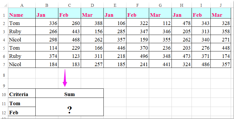
Saya memiliki berbagai data yang berisi header baris dan kolom, sekarang, saya ingin mengambil jumlah sel yang memenuhi kriteria header kolom dan baris. Misalnya, untuk menjumlahkan sel yang kriteria kolomnya adalah Tom dan kriteria barisnya adalah Feb seperti gambar berikut yang ditampilkan. Artikel ini, saya akan berbicara tentang beberapa rumus berguna untuk menyelesaikannya.

doc sum kriteria baris kolom 1

Jumlahkan sel berdasarkan kriteria kolom dan baris dengan rumus


panah gelembung kanan biru Jumlahkan sel berdasarkan kriteria kolom dan baris dengan rumus

Di sini, Anda dapat menerapkan rumus berikut untuk menjumlahkan sel berdasarkan kriteria kolom dan baris, lakukan seperti ini:

Masukkan salah satu dari rumus di bawah ini ke dalam sel kosong tempat Anda ingin mengeluarkan hasilnya:

=SUMPRODUCT((A2:A7="Tom")*(B1:J1="Feb")*(B2:J7))

=SUM(IF(B1:J1="Feb",IF(A2:A7="Tom",B2:J7)))

Lalu tekan Shift + Ctrl + Masuk kunci bersama untuk mendapatkan hasilnya, lihat tangkapan layar:

doc sum kriteria baris kolom 2

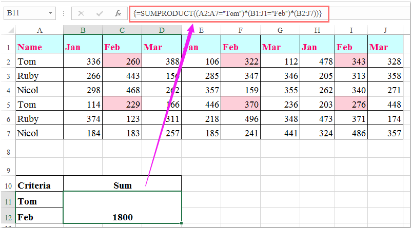
Note: Dalam rumus di atas: Tom dan Februari adalah kriteria kolom dan baris yang didasarkan pada, A2: A7, B1: J1 Apakah tajuk kolom dan tajuk baris berisi kriteria, B2: J7 adalah rentang data yang ingin Anda jumlahkan.

Alat Produktivitas Kantor Terbaik

馃 Kutools AI Ajudan: Merevolusi analisis data berdasarkan: Eksekusi Cerdas   |  Hasilkan Kode  |  Buat Rumus Khusus  |  Analisis Data dan Hasilkan Grafik  |  Aktifkan Fungsi Kutools...
Fitur Populer: Temukan, Sorot, atau Identifikasi Duplikat   |  Hapus Baris Kosong   |  Gabungkan Kolom atau Sel tanpa Kehilangan Data   |   Putaran tanpa Formula ...
Pencarian Super: VLookup Beberapa Kriteria    VLookup Nilai Berganda  |   VLookup di Beberapa Lembar   |   Pencarian Fuzzy ....
Daftar Drop-down Lanjutan: Buat Daftar Drop Down dengan Cepat   |  Daftar Drop Down yang Bergantung   |  Multi-pilih Drop Down List ....
Manajer Kolom: Tambahkan Jumlah Kolom Tertentu  |  Pindahkan Kolom  |  Alihkan Status Visibilitas Kolom Tersembunyi  |  Bandingkan Rentang & Kolom ...
Fitur Unggulan: Fokus Kisi   |  Tampilan Desain   |   Bar Formula Besar    Manajer Buku Kerja & Lembar   |  Perpustakaan Sumberdaya (Teks otomatis)   |  Pemetik tanggal   |  Gabungkan Lembar Kerja   |  Enkripsi/Dekripsi Sel    Kirim Email berdasarkan Daftar   |  Filter Super   |   Filter Khusus (filter tebal/miring/coret...) ...
15 Perangkat Teratas12 Teks Tools (Tambahkan Teks, Hapus Karakter, ...)   |   50 + Grafik jenis (Gantt Chart, ...)   |   40+ Praktis Rumus (Hitung usia berdasarkan ulang tahun, ...)   |   19 Insersi Tools (Masukkan Kode QR, Sisipkan Gambar dari Jalur, ...)   |   12 Konversi Tools (Angka ke Kata, Konversi Mata Uang, ...)   |   7 Gabungkan & Pisahkan Tools (Lanjutan Gabungkan Baris, Pisahkan Sel, ...)   |   ... dan banyak lagi

Tingkatkan Keterampilan Excel Anda dengan Kutools for Excel, dan Rasakan Efisiensi yang Belum Pernah Ada Sebelumnya. Kutools for Excel Menawarkan Lebih dari 300 Fitur Lanjutan untuk Meningkatkan Produktivitas dan Menghemat Waktu.  Klik Di Sini untuk Mendapatkan Fitur yang Paling Anda Butuhkan...

Deskripsi Produk


Tab Office Membawa antarmuka Tab ke Office, dan Membuat Pekerjaan Anda Jauh Lebih Mudah

  • Aktifkan pengeditan dan pembacaan tab di Word, Excel, PowerPoint, Publisher, Access, Visio, dan Project.
  • Buka dan buat banyak dokumen di tab baru di jendela yang sama, bukan di jendela baru.
  • Meningkatkan produktivitas Anda sebesar 50%, dan mengurangi ratusan klik mouse untuk Anda setiap hari!
Comments (17)
No ratings yet. Be the first to rate!
This comment was minimized by the moderator on the site
Brilliant!

The function =SUM(IF(B1:J1="Feb",IF(A2:A7="Tom",B2:J7))) is a great X & Y summation tool.
I would not have thought this logic out on my own.
In fact i took me a minute to deconstruction the operations.

Thank you
This comment was minimized by the moderator on the site
My data that I am trying to retrieve is in a table. Would this impact the result at all? I have:

=SUM(IF('[Primary Controller Active Project Database (KC notes)1.xlsx]Active Project Tracking'!$B2:$B66=X2,IF('[Primary Controller Active Project Database (KC notes)1.xlsx]Active Project Tracking'!$A1:$AV1=AH10,'[Primary Controller Active Project Database (KC notes)1.xlsx]Active Project Tracking'!$H$2:$AV$66)))

So I think the equivalent would be if you did your information above, but in a table in a different workbook. Thoughts?
This comment was minimized by the moderator on the site
If there were negatives in the matrix and you only wanted to include the positives, what would you do? 
I tried to do something like this:

=SUMPRODUCT((Column = Criteria)* ( Row = Criteria) * (second column = Criteria) * (Matrix) * (Matrix >0))

This comment was minimized by the moderator on the site
Is there a way to do this but instead of writing "Tom" & "Feb" in the formula, you are able to reference the criteria cells e.g.A11 & A12?
This comment was minimized by the moderator on the site
Hello, Rianna,Yest, as you said, you can use the cell references to replace the text in the formula, such as:
=SUMPRODUCT((A2:A7=A2)*(B1:J1=C1)*(B2:J7))
=SUM(IF(B1:J1=C1,IF(A2:A7=A2,B2:J7)))
This comment was minimized by the moderator on the site
In the above example which formula should I use if I wanted calculate the sum of the amounts earned by Tom Ruby & Nicol in March?
This comment was minimized by the moderator on the site
Hello, Nabar,To get the result you want, please apply the below formula:=SUMPRODUCT(((A2:A7="Tom")+(A2:A7="Nicol")+(A2:A7="Ruby"))*(B1:J1="Mar")*(B2:J7))
Please try, hope it can help you!
This comment was minimized by the moderator on the site
Hello Skyyang,
Thank you for your response. I tried the formula you suggested but I am not getting the right answer. Probably I wasn't able to put my query correctly. Let me try again I have a spreadsheet with data with daily calculation, I have numbered the first row 1,2,3,4.....132. 2nd, 3rd 4th &5th rows has table headings. The first column has line no's numbered 1, 2,3,.....3005 starting from row 6,range B6:EF3005 has data filled in on everyday basis. In second sheet i have a table in which I want to apply a formula which will look up two line numbers fed in two different rows and calculate the sum from the range B6: EF3005 from the data spreadsheet between the two line numbers from a certain column viz sum of values in column 15 between rows (line No's) 50 & 85.
This comment was minimized by the moderator on the site
Is there a way to make this work with wildcard characters? I'd like to use it on everything starting with certain characters, but with (a fixed number of) undefined characters at the end, i.e. =SUM(IF(B1:J1="Fe*",IF(A2:A7="To*",B2:J7)))
This comment was minimized by the moderator on the site
Should anyone have the same question, this is how I solved it (in Google Sheets, not tested in Excel):

=ArrayFormula(SUM(IF(regexmatch(O5:W5,"^Fe."),IF(regexmatch(N6:N11,"^To."),O6:W11))))

Note that the IF function does not support wildcard characters and that for regexmatch the wildcards are different and can be found here: https://github.com/google/re2/blob/master/doc/syntax.txt
In this particular instance, I used ^ to indicate that Fe & Tom occur at the beginning of text and . to allow for any following character (* would mean zero or more of the previous character, e.g. Fe* would only look for instances with 1 or more "e"s after F)
This comment was minimized by the moderator on the site
I tried to create a formula to calculate if the D12 is blank, it will calculate from K12 to AH12 but it seems this part ' regexmatch(D12,"")' is not working
ArrayFormula(SUM(IF(regexmatch(D12,""),K12:AH12)))
This comment was minimized by the moderator on the site
Thank you so much! You made my day!! @TeSageDS
This comment was minimized by the moderator on the site
how would you do this same formula if you wanted to sum both Feb and March together? please help! thanks

=SUMPRODUCT((A2:A7="Tom")*(B1:J1="Feb")*(B2:J7))
This comment was minimized by the moderator on the site
Hello,Angela,
To solve your problem, you just need to apply the below formula, please try it.

=SUMPRODUCT((A2:A7="Tom")*((B1:J1="Feb")+(B1:J1="Mar"))*(B2:J7)).

Hope it can help you!
This comment was minimized by the moderator on the site
Brilliant
This comment was minimized by the moderator on the site
Worth pointing out that of the two formulas provided above you do not need to enter the SUMPRODUCT formula with Ctrl + Shift + Enter. It will work perfectly well without it.
This comment was minimized by the moderator on the site
Awesome, this is the one what i was looking for. thanks for the help
There are no comments posted here yet
Please leave your comments in English
Posting as Guest
Rate this post:
0   Characters
Suggested Locations