Loncat ke daftar isi utama

Bagaimana cara menyorot nilai terdekat dalam daftar ke nomor tertentu di Excel?

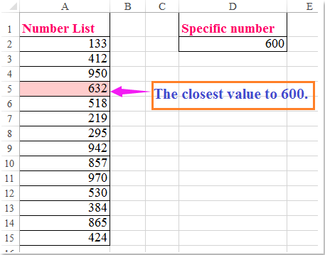
Misalkan, Anda memiliki daftar nomor, sekarang, Anda mungkin ingin menyorot nilai terdekat atau beberapa terdekat berdasarkan nomor tertentu seperti gambar berikut yang ditampilkan. Di sini, artikel ini dapat membantu Anda menyelesaikan tugas ini dengan mudah.

doc sorot nilai terdekat 1
doc sorot nilai terdekat 2

Sorot nilai n terdekat atau terdekat ke angka tertentu dengan Conditional Formatting


panah gelembung kanan biru Sorot nilai n terdekat atau terdekat ke angka tertentu dengan Conditional Formatting

Untuk menyoroti nilai terdekat berdasarkan angka yang diberikan, lakukan hal berikut:

1. Pilih daftar nomor yang ingin Anda sorot, lalu klik Beranda > Format Bersyarat > Aturan baru, lihat tangkapan layar:

doc sorot nilai terdekat 3

2. di Aturan Pemformatan Baru kotak dialog, lakukan operasi berikut:

(1.) Klik Gunakan rumus untuk menentukan sel mana yang akan diformat bawah Pilih Jenis Aturan kotak daftar;

(2.) Di Memformat nilai yang rumus ini benar kotak teks, masukkan rumus ini: =ABS(A2-$D$2)=MIN(ABS($A$2:$A$15-$D$2)) (A2 adalah sel pertama dalam daftar data Anda, D2 adalah angka yang akan Anda bandingkan, A2: A15 adalah daftar nomor yang ingin Anda sorot nilai terdekatnya.)

doc sorot nilai terdekat 4

3. Lalu klik dibentuk tombol untuk membuka Format Cells kotak dialog, di bawah Mengisi tab, pilih satu warna yang Anda suka, lihat tangkapan layar:

doc sorot nilai terdekat 5

4. Dan kemudian klik OK > OK untuk menutup dialog, nilai terdekat ke nomor tertentu telah disorot sekaligus, lihat tangkapan layar:

doc sorot nilai terdekat 6

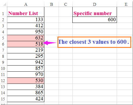
Tips: Jika Anda ingin menyorot 3 nilai yang paling dekat dengan nilai yang diberikan, Anda dapat menerapkan rumus ini di Format Bersyarat, =ISNUMBER(MATCH(ABS($D$2-A2),SMALL(ABS($D$2-$A$2:$A$15),ROW($1:$3)),0)), lihat tangkapan layar:

doc sorot nilai terdekat 7

Note: Dalam rumus di atas: A2 adalah sel pertama dalam daftar data Anda, D2 adalah angka yang akan Anda bandingkan, A2: A15 adalah daftar nomor yang ingin Anda sorot nilai terdekatnya, $ 1: $ 3 menunjukkan bahwa tiga nilai terdekat akan disorot. Anda dapat mengubahnya sesuai kebutuhan Anda.

Alat Produktivitas Kantor Terbaik

馃 Kutools AI Ajudan: Merevolusi analisis data berdasarkan: Eksekusi Cerdas   |  Hasilkan Kode  |  Buat Rumus Khusus  |  Analisis Data dan Hasilkan Grafik  |  Aktifkan Fungsi Kutools...
Fitur Populer: Temukan, Sorot, atau Identifikasi Duplikat   |  Hapus Baris Kosong   |  Gabungkan Kolom atau Sel tanpa Kehilangan Data   |   Putaran tanpa Formula ...
Pencarian Super: VLookup Beberapa Kriteria    VLookup Nilai Berganda  |   VLookup di Beberapa Lembar   |   Pencarian Fuzzy ....
Daftar Drop-down Lanjutan: Buat Daftar Drop Down dengan Cepat   |  Daftar Drop Down yang Bergantung   |  Multi-pilih Drop Down List ....
Manajer Kolom: Tambahkan Jumlah Kolom Tertentu  |  Pindahkan Kolom  |  Alihkan Status Visibilitas Kolom Tersembunyi  |  Bandingkan Rentang & Kolom ...
Fitur Unggulan: Fokus Kisi   |  Tampilan Desain   |   Bar Formula Besar    Manajer Buku Kerja & Lembar   |  Perpustakaan Sumberdaya (Teks otomatis)   |  Pemetik tanggal   |  Gabungkan Lembar Kerja   |  Enkripsi/Dekripsi Sel    Kirim Email berdasarkan Daftar   |  Filter Super   |   Filter Khusus (filter tebal/miring/coret...) ...
15 Perangkat Teratas12 Teks Tools (Tambahkan Teks, Hapus Karakter, ...)   |   50 + Grafik jenis (Gantt Chart, ...)   |   40+ Praktis Rumus (Hitung usia berdasarkan ulang tahun, ...)   |   19 Insersi Tools (Masukkan Kode QR, Sisipkan Gambar dari Jalur, ...)   |   12 Konversi Tools (Angka ke Kata, Konversi Mata Uang, ...)   |   7 Gabungkan & Pisahkan Tools (Lanjutan Gabungkan Baris, Pisahkan Sel, ...)   |   ... dan banyak lagi

Tingkatkan Keterampilan Excel Anda dengan Kutools for Excel, dan Rasakan Efisiensi yang Belum Pernah Ada Sebelumnya. Kutools for Excel Menawarkan Lebih dari 300 Fitur Lanjutan untuk Meningkatkan Produktivitas dan Menghemat Waktu.  Klik Di Sini untuk Mendapatkan Fitur yang Paling Anda Butuhkan...

Deskripsi Produk


Tab Office Membawa antarmuka Tab ke Office, dan Membuat Pekerjaan Anda Jauh Lebih Mudah

  • Aktifkan pengeditan dan pembacaan tab di Word, Excel, PowerPoint, Publisher, Access, Visio, dan Project.
  • Buka dan buat banyak dokumen di tab baru di jendela yang sama, bukan di jendela baru.
  • Meningkatkan produktivitas Anda sebesar 50%, dan mengurangi ratusan klik mouse untuk Anda setiap hari!
Comments (8)
No ratings yet. Be the first to rate!
This comment was minimized by the moderator on the site
=ABS(A2-$D$2)=MIN(ABS($A$2:$A$15-$D$2)) 写邪薪薪邪褟 褎芯褉屑褍谢邪 薪械 褉邪斜芯褌邪械褌. 袩褉芯斜芯胁邪谢 exel 2010 懈 2013. 袝褋谢懈 懈褋锌芯谢褜蟹芯胁邪褌褜 胁褌芯褉褍褞 褎芯褉屑褍谢褍, 褉褍谐邪械褌褋褟 薪邪 芯褕懈斜泻褍.
This comment was minimized by the moderator on the site
Hello friend,

Sorry to hear that. But I did try the two formulas and they both work perfectly. Please see the screenshots.
Here is the tip. Please make sure you choose the right range, in my case here, it is A2:A15. Then click Home > Conditional Formatting to set up the rules. Please have a try. If the problem still remains, please provide me with more details so I can help you. Have a nice day.

Sincerely,
Mandy
This comment was minimized by the moderator on the site
Hi, das hilft mir bereits sehr weiter, danke!Gibt es aber auch eine M枚glichkeit, die Formel aus Schritt 2 ohne "$"-Zeichen zu verwenden? Das w眉rde das Kopieren der bedingten Formatierung erleichtern...
This comment was minimized by the moderator on the site
What if data is over column and not in a row?
This comment was minimized by the moderator on the site
This is useful, but how would I do the following please. Text is in Col A, the number range is in Col B: when the average has been found using the above method and is thus highlighted, I need the corresponding cell in Col A to also highlight.

Thank you
This comment was minimized by the moderator on the site
Were you able to figure this out? I would also like to know about expanding the format to the remaining row.
This comment was minimized by the moderator on the site
Hi! I am very thankfull to u for this as this solved my problem for a presentation to a client. However I am looking for something more for my future presentations. like when u say highlight 3 closest(n) values i want to highlight them as: 1) the most closest with Green. 2) the least closest in red and the 3) value which is between most and least closest in yellow. Can u please help me to achieve this. As per the example my d2 value is live updating every minute so i want to know where exactly my d2 value lies on scale of a range(eg. Number list). This will add a brand finish to my presentations. Point to note i am using excel 2007 as many of my clients are still using the same. Just to avoid any compatibility issues i avoid latest versions. Thanks in advance and many regards. :)
This comment was minimized by the moderator on the site
An excellent resource for highlighting the closest value. Since the logic is same , won't it work in Google Sheets? Anyway it is not working in Google Sheets. Would be obliged if you could please clarify!
There are no comments posted here yet
Please leave your comments in English
Posting as Guest
Rate this post:
0   Characters
Suggested Locations