Bagaimana cara menyorot sel atau baris dengan kotak centang di Excel?
Seperti gambar di bawah ini yang ditampilkan, Anda perlu menyorot baris atau sel dengan kotak centang. Saat kotak centang dicentang, baris atau sel tertentu akan disorot secara otomatis. Tapi bagaimana cara mencapainya di Excel? Artikel ini akan menunjukkan dua metode untuk mencapainya.

Sorot sel atau baris dengan kotak centang dengan Pemformatan Bersyarat
Sorot sel atau baris dengan kotak centang dengan kode VBA
Sorot sel atau baris dengan kotak centang dengan Pemformatan Bersyarat
Anda dapat membuat aturan Pemformatan Bersyarat untuk menyorot sel atau baris dengan kotak centang di Excel. Silakan lakukan sebagai berikut.
Tautkan semua kotak centang ke sel tertentu
1. Anda perlu memasukkan kotak centang ke dalam sel satu per satu secara manual dengan mengklik Pengembang > Menyisipkan > Kotak cek (Kontrol Formulir).
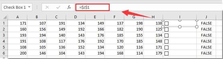
2. Sekarang kotak centang telah disisipkan ke sel di kolom I. Pilih kotak centang pertama di I1, masukkan rumus = $ J1 ke dalam bilah rumus, lalu tekan Enter kunci.
jenis: Jika Anda tidak ingin memiliki nilai yang terkait di sel yang berdekatan dengan kotak centang, Anda dapat menautkan kotak centang ke sel lembar kerja lain seperti = Sheet3! $ E1.
2. Ulangi langkah 1 sampai semua kotak centang ditautkan ke sel atau sel yang berdekatan di lembar kerja lain.
Note: Semua sel yang ditautkan harus berurutan dan terletak di kolom yang sama.
Buat aturan Pemformatan Bersyarat
Sekarang Anda perlu membuat aturan Pemformatan Bersyarat sebagai berikut langkah demi langkah.
1. Pilih baris yang perlu Anda sorot dengan kotak centang, lalu klik Format Bersyarat > Aturan baru bawah Beranda tab. Lihat tangkapan layar:

2. Dalam Aturan Pemformatan Baru kotak dialog, Anda perlu:
2.1 Pilih Gunakan rumus untuk menentukan sel mana yang akan diformat pilihan dalam Pilih Jenis Aturan kotak;
2.2 Memasukkan rumus = JIKA ($ J1 = BENAR, BENAR, SALAH) ke dalam Memformat nilai yang rumus ini benar kotak;
Or = JIKA (Sheet3! $ E1 = BENAR, BENAR, SALAH) jika kotak centang ditautkan ke lembar kerja lain.
2.3 Klik tombol dibentuk tombol untuk menentukan warna yang disorot untuk baris;
2.4 Klik tombol OK tombol. Lihat tangkapan layar:

Note: Dalam rumusnya, $ J1 or $ E1 adalah sel tertaut pertama untuk kotak centang, dan pastikan referensi sel telah diubah menjadi absolut kolom (J1> $ J1 or E1> $ E1).
Sekarang aturan Conditional Formatting dibuat. Saat mencentang kotak centang, baris yang sesuai akan disorot secara otomatis saat screenshot bellow ditampilkan.

Sorot sel atau baris dengan kotak centang dengan kode VBA
Kode VBA berikut juga dapat membantu Anda menyorot sel atau baris dengan kotak centang di Excel. Silakan lakukan sebagai berikut.
1. Pada lembar kerja Anda perlu menyorot sel atau baris dengan kotak centang. Klik kanan file Tab Lembar dan pilih Lihat kode dari menu klik kanan untuk membuka Microsoft Visual Basic untuk Aplikasi jendela.
2. Kemudian salin dan tempel kode VBA di bawah ini ke jendela Kode.
Kode VBA: Sorot baris dengan kotak centang di Excel
Sub AddCheckBox()
Dim xCell As Range
Dim xRng As Range
Dim I As Integer
Dim xChk As CheckBox
On Error Resume Next
InputC:
    Set xRng = Application.InputBox("Please select the column range to insert checkboxes:", "Kutools for Excel", Selection.Address, , , , , 8)
If xRng Is Nothing Then Exit Sub
If xRng.Columns.Count > 1 Then
    MsgBox "The selected range should be a single column", vbInformation, "Kutools fro Excel"
    GoTo InputC
Else
    If xRng.Columns.Count = 1 Then
        For Each xCell In xRng
            With ActiveSheet.CheckBoxes.Add(xCell.Left, _
               xCell.Top, xCell.Width = 15, xCell.Height = 12)
               .LinkedCell = xCell.Offset(, 1).Address(External:=False)
               .Interior.ColorIndex = xlNone
               .Caption = ""
               .Name = "Check Box " & xCell.Row
            End With
            xRng.Rows(xCell.Row).Interior.ColorIndex = xlNone
        Next
    End If
    With xRng
     .Rows.RowHeight = 16
    End With
    xRng.ColumnWidth = 5#
    xRng.Cells(1, 1).Offset(0, 1).Select
    For Each xChk In ActiveSheet.CheckBoxes
      xChk.OnAction = ActiveSheet.Name + ".InsertBgColor"
    Next
End If
End Sub

Sub InsertBgColor()
Dim xName As Integer
Dim xChk As CheckBox
For Each xChk In ActiveSheet.CheckBoxes
  xName = Right(xChk.Name, Len(xChk.Name) - 10)
  If (xName = Range(xChk.LinkedCell).Row) Then
   If (Range(xChk.LinkedCell) = "True") Then
    Range("A" & xName, Range(xChk.LinkedCell).Offset(0, -2)).Interior.ColorIndex = 6
   Else
    Range("A" & xName, Range(xChk.LinkedCell).Offset(0, -2)).Interior.ColorIndex = xlNone
   End If
  End If
Next
End Sub
3. tekan F5 kunci untuk menjalankan kode. (Note: Anda harus meletakkan kursor ke bagian pertama kode untuk menerapkan tombol F5) di popping up Kutools untuk Excel kotak dialog, pilih kisaran yang ingin Anda sisipkan kotak centang, dan kemudian klik OK tombol. Di sini saya memilih rentang I1: I6. Lihat tangkapan layar:

4. Kemudian kotak centang dimasukkan ke dalam sel yang dipilih. Centang salah satu kotak centang, baris yang sesuai akan disorot secara otomatis seperti gambar di bawah ini.

Terkait artikel:
- Bagaimana cara mengubah nilai sel atau warna tertentu saat kotak centang dicentang di Excel?
- Bagaimana cara memasukkan cap tanggal ke dalam sel jika mencentang kotak centang di Excel?
- Bagaimana cara membuat kotak centang dicentang berdasarkan nilai sel di Excel?
- Bagaimana cara memfilter data berdasarkan kotak centang di Excel?
- Bagaimana cara menyembunyikan kotak centang saat baris disembunyikan di Excel?
- Bagaimana cara membuat daftar drop-down dengan beberapa kotak centang di Excel?
Alat Produktivitas Kantor Terbaik
Tingkatkan Keterampilan Excel Anda dengan Kutools for Excel, dan Rasakan Efisiensi yang Belum Pernah Ada Sebelumnya. Kutools for Excel Menawarkan Lebih dari 300 Fitur Lanjutan untuk Meningkatkan Produktivitas dan Menghemat Waktu. Klik Di Sini untuk Mendapatkan Fitur yang Paling Anda Butuhkan...
")
Tab Office Membawa antarmuka Tab ke Office, dan Membuat Pekerjaan Anda Jauh Lebih Mudah
- Aktifkan pengeditan dan pembacaan tab di Word, Excel, PowerPoint, Publisher, Access, Visio, dan Project.
- Buka dan buat banyak dokumen di tab baru di jendela yang sama, bukan di jendela baru.
- Meningkatkan produktivitas Anda sebesar 50%, dan mengurangi ratusan klik mouse untuk Anda setiap hari!
")