Loncat ke daftar isi utama

Bagaimana cara menerapkan pencarian pemformatan bersyarat untuk beberapa kata di Excel?

doc sorotan berisi kata apa saja 1

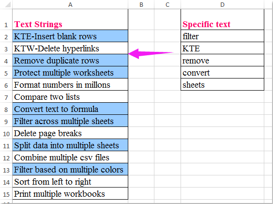
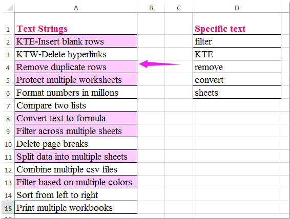
Mungkin mudah bagi kita untuk menyorot baris berdasarkan nilai tertentu, artikel ini, saya akan berbicara tentang cara menyorot sel di kolom A tergantung apakah mereka ditemukan di kolom D, yang berarti, jika konten sel berisi teks apa pun di daftar tertentu, lalu sorot sebagai tangkapan layar kiri yang ditampilkan.

Pemformatan bersyarat untuk menyorot sel berisi salah satu dari beberapa nilai

Filter sel berisi nilai tertentu dan sorot sekaligus


Pemformatan bersyarat untuk menyorot sel berisi salah satu dari beberapa nilai

Bahkan, Format Bersyarat dapat membantu Anda menyelesaikan pekerjaan ini, lakukan dengan langkah-langkah berikut:

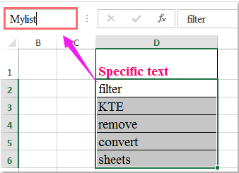
1. Pertama, buat nama rentang untuk daftar kata tertentu, pilih teks sel dan masukkan nama rentang Daftarku (Anda dapat mengganti nama sesuai kebutuhan) menjadi Nama kotak, dan tekan Enter kunci, lihat tangkapan layar:

doc sorotan berisi kata apa saja 2

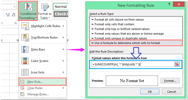
2. Kemudian pilih sel yang ingin Anda sorot, dan klik Beranda > Format Bersyarat > Aturan baru, Dalam Aturan Pemformatan Baru kotak dialog, selesaikan operasi di bawah ini:

(1.) Klik Gunakan rumus untuk menentukan sel mana yang akan diformat bawah Pilih Jenis Aturan kotak daftar;

(2.) Lalu masukkan rumus ini: = SUM (COUNTIF (A2, "*" & Daftar Saya & "*")) (A2 adalah sel pertama dari rentang yang ingin Anda sorot, Daftarku adalah nama rentang yang telah Anda buat pada langkah 1) ke dalam Memformat nilai yang rumus ini benar kolom tulisan;

(3.) Lalu klik dibentuk .

doc sorotan berisi kata apa saja 3

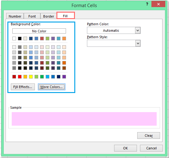
3. Pergi ke Format Cells kotak dialog, dan pilih satu warna untuk menyorot sel di bawah Mengisi tab, lihat tangkapan layar:

doc sorotan berisi kata apa saja 4

4. Dan kemudian klik OK > OK untuk menutup dialog, semua sel yang berisi salah satu dari daftar nilai sel tertentu disorot sekaligus, lihat tangkapan layar:

doc sorotan berisi kata apa saja 5


Filter sel berisi nilai tertentu dan sorot sekaligus

Jika Anda memiliki Kutools untuk Excel, Dengan yang Filter Super utilitas, Anda dapat dengan cepat memfilter sel yang berisi nilai teks tertentu, lalu menyorotnya sekaligus.

Kutools untuk Excel : dengan lebih dari 300 add-in Excel yang praktis, gratis untuk dicoba tanpa batasan dalam 30 hari. 

Setelah menginstal Kutools untuk Excel, lakukan hal berikut:

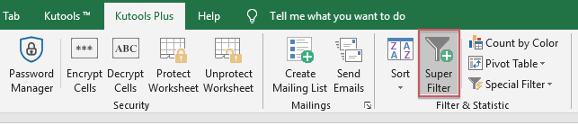
1. Klik Kutools Ditambah > Filter Super, lihat tangkapan layar:

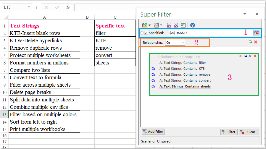
2. di Filter Super panel, lakukan operasi berikut:

  • (1.) Periksa Ditentukan pilihan, lalu klik doc sorotan berisi kata apa saja 11 tombol untuk memilih rentang data yang ingin Anda filter;
  • (2.) Pilih hubungan di antara kriteria filter yang Anda butuhkan;
  • (3.) Kemudian tentukan kriteria di kotak daftar kriteria.

doc sorotan berisi kata apa saja 8

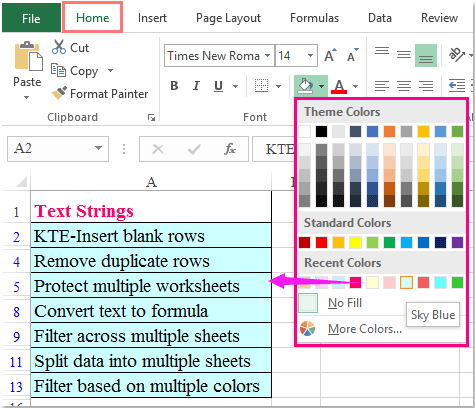
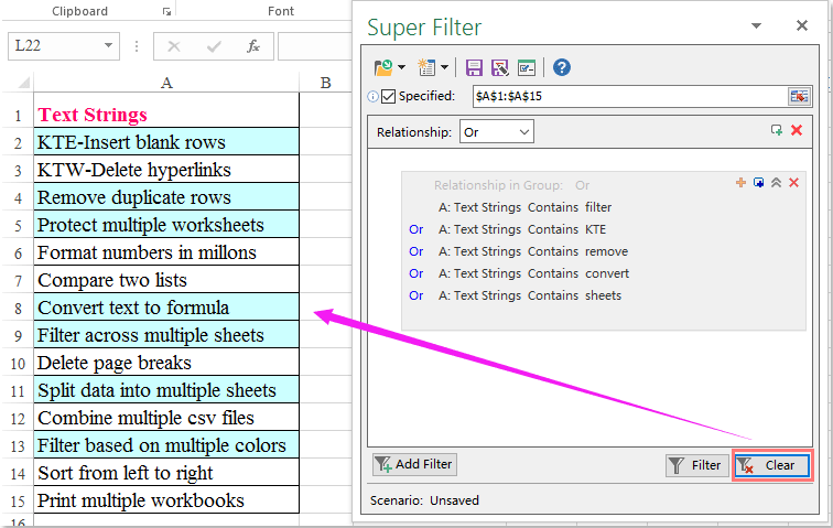
3. Setelah mengatur kriteria, klik Filter untuk memfilter sel berisi nilai spesifik yang Anda butuhkan. Dan kemudian pilih satu warna isian untuk sel yang dipilih di bawah Beranda tab, lihat tangkapan layar:

doc sorotan berisi kata apa saja 9

4. Dan semua sel berisi nilai tertentu disorot, sekarang, Anda dapat membatalkan filter dengan mengklik Hapus tombol, lihat tangkapan layar:

doc sorotan berisi kata apa saja 10

Klik Unduh dan uji coba gratis Kutools untuk Excel Sekarang!


Demo: Sel filter berisi nilai tertentu dan sorot sekaligus

Kutools untuk Excel: dengan lebih dari 300 add-in Excel yang praktis, gratis untuk dicoba tanpa batasan dalam 30 hari. Unduh dan uji coba gratis Sekarang!

Alat Produktivitas Kantor Terbaik

🤖 Kutools AI Ajudan: Merevolusi analisis data berdasarkan: Eksekusi Cerdas   |  Hasilkan Kode  |  Buat Rumus Khusus  |  Analisis Data dan Hasilkan Grafik  |  Aktifkan Fungsi Kutools...
Fitur Populer: Temukan, Sorot, atau Identifikasi Duplikat   |  Hapus Baris Kosong   |  Gabungkan Kolom atau Sel tanpa Kehilangan Data   |   Putaran tanpa Formula ...
Pencarian Super: VLookup Beberapa Kriteria    VLookup Nilai Berganda  |   VLookup di Beberapa Lembar   |   Pencarian Fuzzy ....
Daftar Drop-down Lanjutan: Buat Daftar Drop Down dengan Cepat   |  Daftar Drop Down yang Bergantung   |  Multi-pilih Drop Down List ....
Manajer Kolom: Tambahkan Jumlah Kolom Tertentu  |  Pindahkan Kolom  |  Alihkan Status Visibilitas Kolom Tersembunyi  |  Bandingkan Rentang & Kolom ...
Fitur Unggulan: Fokus Kisi   |  Tampilan Desain   |   Bar Formula Besar    Manajer Buku Kerja & Lembar   |  Perpustakaan Sumberdaya (Teks otomatis)   |  Pemetik tanggal   |  Gabungkan Lembar Kerja   |  Enkripsi/Dekripsi Sel    Kirim Email berdasarkan Daftar   |  Filter Super   |   Filter Khusus (filter tebal/miring/coret...) ...
15 Perangkat Teratas12 Teks Tools (Tambahkan Teks, Hapus Karakter, ...)   |   50 + Grafik jenis (Gantt Chart, ...)   |   40+ Praktis Rumus (Hitung usia berdasarkan ulang tahun, ...)   |   19 Insersi Tools (Masukkan Kode QR, Sisipkan Gambar dari Jalur, ...)   |   12 Konversi Tools (Angka ke Kata, Konversi Mata Uang, ...)   |   7 Gabungkan & Pisahkan Tools (Lanjutan Gabungkan Baris, Pisahkan Sel, ...)   |   ... dan banyak lagi

Tingkatkan Keterampilan Excel Anda dengan Kutools for Excel, dan Rasakan Efisiensi yang Belum Pernah Ada Sebelumnya. Kutools for Excel Menawarkan Lebih dari 300 Fitur Lanjutan untuk Meningkatkan Produktivitas dan Menghemat Waktu.  Klik Di Sini untuk Mendapatkan Fitur yang Paling Anda Butuhkan...

Deskripsi Produk


Tab Office Membawa antarmuka Tab ke Office, dan Membuat Pekerjaan Anda Jauh Lebih Mudah

  • Aktifkan pengeditan dan pembacaan tab di Word, Excel, PowerPoint, Publisher, Access, Visio, dan Project.
  • Buka dan buat banyak dokumen di tab baru di jendela yang sama, bukan di jendela baru.
  • Meningkatkan produktivitas Anda sebesar 50%, dan mengurangi ratusan klik mouse untuk Anda setiap hari!
Comments (34)
Rated 4.5 out of 5 · 1 ratings
This comment was minimized by the moderator on the site
=SUMPRODUCT(--ISNUMBER(SEARCH(IF(Mylist<>"",Mylist),A2)))>0
How to Format whole row in this formula
This comment was minimized by the moderator on the site
THANK YOU VERY MUCH, YOU SAVED A LOT OF TIME OF ME.
This comment was minimized by the moderator on the site
Hello, Akash,
Glad it can help you!
Have a good new year! 😄
This comment was minimized by the moderator on the site
Above formula not working, coz , My condition (i.e if my list is blank). And if my list is remaining blank excel formatting all cells. Help me.
This comment was minimized by the moderator on the site
Hello, Akash,
If your data list contains blank cell, please apply the below formula into the Conditional Formatting:
=SUMPRODUCT(--ISNUMBER(SEARCH(IF(Mylist<>"",Mylist),A2)))>0
Please have a try, hope it can help you!
This comment was minimized by the moderator on the site
I want to format whole Row. In this formula how to format whole Row.
This comment was minimized by the moderator on the site
I want to format only the text contained in my list. I do not want to format if my list (one or two cell of my list) is blank
This comment was minimized by the moderator on the site
Hello, AKASH
To solve your problem, the following article may help you:
https://www.extendoffice.com/documents/excel/2499-excel-conditional-formatting-ignore-blank-zero.html

Please have a try, thank you!
This comment was minimized by the moderator on the site
Greetings!

I am trying to use a range of words in a row, from another sheet.
My formula looks like this:

=Info!=SUM(COUNTIF($A1,"*"&LGreen&"*"))

"Info" is the sheet, "LGreen" is the row of words i want to use, and the words start at A1 in "Info" sheet.

But i still get "There is a problem with this formula.......
Does it matter if the words are in a row/column? And how do i make that change in the formula?
I would like to use the whole row (continuous), so that i can put in more words later on.
If not, i can select specific range/cells, as long as i understand whats wrong x)

Thanks in advance!
This comment was minimized by the moderator on the site
Hello, Sykopaten

In fact, you just need follow the method in the article, in the first step, you should create a range name for your data list in aother sheet, which can be applied to the entire workbook. And then use the formula: =SUM(COUNTIF(A2,"*"&Mylist&"*")) into the conditional formatting of the worksheet you want to highlihgt the cells.

Or you can insert your excel file as attachment here for us to check.

Thank you!
This comment was minimized by the moderator on the site
Thank you so much to the reply! This surely helped a lot!
Have a great new year! :D
This comment was minimized by the moderator on the site
Hello, Sykopaten,
Glad it can help you!
Happy new year!😀
This comment was minimized by the moderator on the site
Can you provide instructions for how to reverse this formula. In the same example, how would you format cells that did NOT contain a word from your keyword list?
Rated 4.5 out of 5
This comment was minimized by the moderator on the site
Hello, Jeff,
To solve your problem, please apply the below formula:
=IF(SUM(COUNTIF(A2,"*"&Mylist&"*"))=1, 0,1)

Please have a try, hope it can help you!
This comment was minimized by the moderator on the site
Consegui, a formula é funcional e adorei!! obrigado!
This comment was minimized by the moderator on the site
Hello,

is the formula sensitive to space?
This comment was minimized by the moderator on the site
I have a List that contains "Numbers" and when I run this formula it only work on "Word/Text". What shall be my approach for numbers? For example, I have two rego ( registration) number for management team eg 1234 and 6789, so my data in A column will contain a lot of different vehicle number, i want to hightlight GREEN only these two regos.
This comment was minimized by the moderator on the site
This is for the "OR" function. How do I go abouts this with the "AND"?

As in I need to highlight ONLY the cells that have all of the list and not just either of the list.
There are no comments posted here yet
Load More
Please leave your comments in English
Posting as Guest
×
Rate this post:
0   Characters
Suggested Locations