Loncat ke daftar isi utama

Bagaimana mengembalikan nilai di sel lain jika sel berisi teks tertentu di Excel?

Seperti contoh di bawah ini, ketika sel E6 berisi nilai "Ya", sel F6 akan secara otomatis diisi dengan nilai "menyetujui". Jika Anda mengubah "Ya" menjadi "Tidak" atau "Netralitas" di E6, nilai di F6 akan segera diubah menjadi "Tolak" atau "Pertimbangkan Kembali". Bagaimana cara yang dapat Anda lakukan untuk mencapainya? Artikel ini mengumpulkan beberapa metode berguna untuk membantu Anda menyelesaikannya dengan mudah.


Kembalikan nilai di sel lain jika sel berisi teks tertentu dengan rumus

Untuk mengembalikan nilai di sel lain jika sel hanya berisi teks tertentu, coba rumus berikut. Misalnya, jika B5 berisi "Ya", maka kembalikan "Setuju" di D5, jika tidak, kembalikan "Tidak memenuhi syarat". Silakan lakukan sebagai berikut.

Pilih D5 dan salin rumus di bawah ini ke dalamnya dan tekan Enter kunci. Lihat tangkapan layar:

Formula: Kembalikan nilai di sel lain jika sel berisi teks tertentu

= JIKA (ISNUMBER (CARI ("Yes",D5)), "Menyetujui","Tidak memenuhi syarat")

Catatan:

1. Dalam rumusnya, "Yes", D5, "menyetujui"Dan"Tidak memenuhi syarat”Menunjukkan bahwa jika sel B5 berisi teks“ Ya ”, sel yang ditentukan akan diisi dengan teks“ setuju ”, jika tidak, akan diisi dengan“ Tidak memenuhi syarat ”. Anda dapat mengubahnya berdasarkan kebutuhan Anda.

2. Untuk mengembalikan nilai dari sel lain (seperti K8 dan K9) berdasarkan nilai sel yang ditentukan, gunakan rumus ini:

= JIKA (ISNUMBER (CARI ("Yes",D5)),K8,K9)

Pilih dengan mudah seluruh baris atau seluruh baris dalam pemilihan berdasarkan nilai sel di kolom tertentu:

Grafik Pilih Sel Spesifik kegunaan Kutools untuk Excel dapat membantu Anda dengan cepat memilih seluruh baris atau seluruh baris dalam pemilihan berdasarkan nilai sel tertentu di kolom tertentu di Excel.  Unduh fitur lengkap jejak gratis 60 hari dari Kutools untuk Excel sekarang!


Kembalikan nilai di sel lain jika sel berisi teks berbeda dengan rumus

Bagian ini akan menunjukkan kepada Anda rumus untuk mengembalikan nilai di sel lain jika sel berisi teks berbeda di Excel.

1. Anda perlu membuat tabel dengan nilai spesifik dan mengembalikan nilai yang terletak secara terpisah dalam dua kolom. Lihat tangkapan layar:

2. Pilih sel kosong untuk mengembalikan nilai, ketikkan rumus di bawah ini ke dalamnya dan tekan Enter kunci untuk mendapatkan hasil. Lihat tangkapan layar:

Formula: Kembalikan nilai di sel lain jika sel berisi teks berbeda

= VLOOKUP (E6,B5: C7,2,SALAH)

Catatan:

Dalam formula tersebut, E6 adalah sel berisi nilai spesifik yang akan Anda kembalikan berdasarkan nilai, B5: C7 adalah rentang kolom yang berisi nilai spesifik dan nilai kembalian, yaitu 2 angka berarti bahwa nilai-nilai kembali yang terletak di kolom kedua dalam rentang tabel.

Mulai sekarang, saat mengubah nilai di E6 ke nilai tertentu, nilai yang sesuai akan segera dikembalikan di F6.


Mengembalikan nilai dengan mudah di sel lain jika sel berisi teks berbeda

Sebenarnya kamu bisa menyelesaikan masalah di atas dengan cara yang lebih mudah. Itu Cari nilai dalam daftar kegunaan Kutools untuk Excel dapat membantu Anda mencapainya hanya dengan beberapa klik tanpa mengingat rumus.

1. Sama seperti metode di atas, Anda juga perlu membuat tabel dengan nilai tertentu dan mengembalikan nilai yang ditempatkan secara terpisah dalam dua kolom.

2. Pilih sel kosong untuk menampilkan hasilnya (di sini saya pilih F6), lalu klik Kutools > Pembantu Formula > Pembantu Formula. Lihat tangkapan layar:

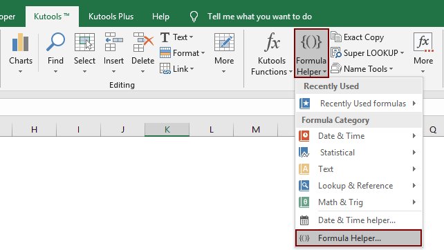
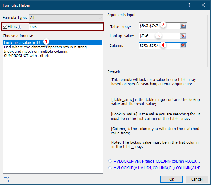
3. Dalam Pembantu Formula kotak dialog, konfigurasikan sebagai berikut:

  • 3.1 Dalam Pilih rumus kotak, temukan dan pilih Cari nilai dalam daftar;
    Tips: Anda dapat memeriksa Filter kotak, masukkan kata tertentu ke dalam kotak teks untuk memfilter rumus dengan cepat.
  • 3.2 Dalam Tabel_array kotak, pilih tabel tanpa header yang telah Anda buat pada langkah 1;
  • 3.2 Dalam Nilai lookup kotak, pilih sel yang berisi nilai spesifik yang akan Anda kembalikan berdasarkan nilai;
  • 3.3 Dalam Kolom kotak, tentukan dari kolom mana Anda akan mengembalikan nilai yang cocok. Atau Anda dapat memasukkan nomor kolom ke dalam kotak teks secara langsung sesuai kebutuhan.
  • 3.4 Klik tombol OK tombol. Lihat tangkapan layar:

Mulai sekarang, saat mengubah nilai di E6 ke nilai tertentu, nilai yang sesuai akan segera dikembalikan di F6. Lihat hasil seperti di bawah ini:

  Jika Anda ingin memiliki uji coba gratis (30 hari) dari utilitas ini, silahkan klik untuk mendownloadnya, lalu lanjutkan untuk menerapkan operasi sesuai langkah di atas.


Kutools untuk Excel - Membantu Anda Selalu Menyelesaikan Pekerjaan Sebelumnya, Memiliki Lebih Banyak Waktu untuk Menikmati Hidup
Apakah Anda sering mengejar ketinggalan dengan pekerjaan, kurangnya waktu untuk diri sendiri dan keluarga?  Kutools untuk Excel dapat membantu Anda untuk menangani 80% Teka-teki Excel dan tingkatkan efisiensi kerja 80%, memberi Anda lebih banyak waktu untuk mengurus keluarga dan menikmati hidup.
300 alat canggih untuk 1500 skenario kerja, buat pekerjaan Anda jauh lebih mudah dari sebelumnya.
Tidak perlu lagi menghafal rumus dan kode VBA, istirahatkan otak Anda mulai sekarang.
Operasi yang rumit dan berulang dapat dilakukan pemrosesan satu kali dalam hitungan detik.
Kurangi ribuan operasi keyboard & mouse setiap hari, ucapkan selamat tinggal pada penyakit akibat kerja sekarang.
Menjadi ahli Excel dalam 3 menit, membantu Anda dengan cepat dikenali dan promosi kenaikan gaji.
110,000 orang yang sangat efektif dan pilihan 300+ perusahaan terkenal di dunia.
Buat $ 39.0 Anda bernilai lebih dari $ 4000.0 dengan pelatihan orang lain.
Uji coba gratis fitur lengkap selama 30 hari. Jaminan Uang Kembali 60 Hari tanpa alasan.

Comments (98)
No ratings yet. Be the first to rate!
This comment was minimized by the moderator on the site
What would I need to add to this formula (Method A) to get a third BLANK option? And where would it go?
Example:
If the cell I'm searching is blank, I would like it to return no value in the other cell. I do not want the "if false" value to populate.
This comment was minimized by the moderator on the site
i want a cell to automatically choose a number based on the drop-down option in the cell before, e.g drop-down, half meal, full meal, if I select half meal drop-down, the next cell should show 50% while the full meal drop-down will reflect 100%. please help
This comment was minimized by the moderator on the site
Hi Josh,
In the cell where you want to output the percentage, enter the following formula and press the Enter key. Hope I can help.
=IF(C15="half meal", "50%", IF(C15="full meal", "100%", ""))
This comment was minimized by the moderator on the site
Is it possible to return a certain value in 1 column based on another?


What I currently have: On a differnt tab (same worksheet):
Column A Column B
Location Name Dept Location Name Location Code
Miami 4455 Miami 123


What I want to happen:
Location Name Dept
Miami 11234455

In Coumn B, I want it to first add a 1, then take what is in Column A, see what is the Location Code on then different tab, insert that location code, and add that to the front of the current data in Column B.

1 + 123 + 4455
This comment was minimized by the moderator on the site
Hi Jen Rader,
You can apply the following formula to get it done.
=IFERROR(1&VLOOKUP(A9,Sheet2!$A$2:$B$5,2, 0)&VLOOKUP(Sheet1!A9,Sheet1!$A$2:$B$5,2, 0),"")
In this formula,
1. A9 is the cell contains the value you want to return values based on;
2. Sheet2 is the tab name contains the "Location Code"; If the tab name contains space, please enclose the tab name in single quotes, such as 'tab name'.
3. Sheet1 is the tab name contains the "Dept";
4. $A$2:$B$5 is the range containing the table data (include both search values and return values ).
See screenshots below:
https://www.extendoffice.com/images/stories/comments/comment-picture-zxm/return1.png
https://www.extendoffice.com/images/stories/comments/comment-picture-zxm/return2.png
This comment was minimized by the moderator on the site
OMG Crystal! You are amazing! Show me your ways! Thank you so much - it worked exactly like I was hoping!
This comment was minimized by the moderator on the site
I am trying to find out the formula to copy the number shown in B2 on cell D2 if the Cell C2 has a letter "S". Can anyone help me?
This comment was minimized by the moderator on the site
Hi Aurora,
Please enter the following formula in cell D2.
=IF(ISNUMBER(SEARCH("S",C2)),B2,"No qualify")
This comment was minimized by the moderator on the site
Bonjour à tous, j'ai un tableau Excel et j'aimerais réaliser via une macro l'opération suivante: si une cellule contient une date, me renvoyer une valeur dans une autre cellule. Pourriez vous m'aider s'il vous plait? Je vous remercie par avance
This comment was minimized by the moderator on the site
STALLS D 25 Palais - Stalls SR
STALLS M 19 Palais - Stalls SR
LOUNGE E 22 Palais - Lounge SR
LOUNGE G 23 Palais - Lounge SL
ORCH K 40 Palais - Orchestra SR
For each line in a spreadsheet I need to evaluate against a table like above and find the value that matches all of the first 3 values.
Normally I would use sumifs for this type of problem but the answer is a text string so it returns 0
This comment was minimized by the moderator on the site
I need a formula that makes column N equal the text “OTO” if column K equals MCS TRAINING how do I do that???
This comment was minimized by the moderator on the site
Hi Abby,Please apply the following formula in the cells of column N:=IF(ISNUMBER(MATCH("MCS TRAINING",K1)),"OTO","NULL")
This comment was minimized by the moderator on the site
Hi - This is my formula that I am working with.  Currently it works, but where B21 is being returned, the value of B21 is a link to another place altogether.  I want to keep the display text but would like to include the link as well.  Can this be done?  =IF(ISNUMBER(SEARCH("DATA_MAPPING",general_report!AJ21)),general_report!B21,"")
This comment was minimized by the moderator on the site
Is it possible to split the return value to a different tab? IE: columns B and C are located on one tab, and values in columns E and F are located on a different tab?
This comment was minimized by the moderator on the site
Hi

Is it possible to populate another cell, not the cell with the formula.

Example
A1 Yes
A2 3
A3 Formula searches A1, Grabs value at A2 and if Yes Paste it in A4
A4 3 
This comment was minimized by the moderator on the site
Hi,
Sorry can't help you with the problem. I suggest you post the problem to the forum below to get help from other Excel enthusiasts.
https://www.extendoffice.com/forum/kutools-for-excel.html 
There are no comments posted here yet
Load More
Please leave your comments in English
Posting as Guest
×
Rate this post:
0   Characters
Suggested Locations