Loncat ke daftar isi utama

Bagaimana cara menghitung nilai unik berdasarkan kolom lain di Excel?

jumlah doc unik dengan kriteria 1

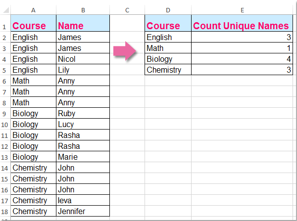
Mungkin umum bagi kita untuk menghitung nilai unik hanya dalam satu kolom, tetapi, dalam artikel ini, saya akan berbicara tentang cara menghitung nilai unik berdasarkan kolom lain. Misalnya, saya memiliki data dua kolom berikut, sekarang, saya perlu menghitung nama-nama unik di kolom B berdasarkan konten kolom A untuk mendapatkan hasil sebagai berikut:

Hitung nilai unik berdasarkan kolom lain dengan rumus array


panah gelembung kanan biru Hitung nilai unik berdasarkan kolom lain dengan rumus array

Untuk mengatasi masalah ini, rumus berikut dapat membantu Anda, lakukan hal berikut:

1. Masukkan rumus ini: =SUMPRODUCT((($A$2:$A$18=D2))/COUNTIFS($A$2:$A$18,$A$2:$A$18&"",$B$2:$B$18,$B$2:$B$18&"")) ke dalam sel kosong tempat Anda ingin meletakkan hasilnya, E2, misalnya. Lalu tekan Ctrl + Shift + Enter kunci bersama untuk mendapatkan hasil yang benar, lihat tangkapan layar:

jumlah doc unik dengan kriteria 2

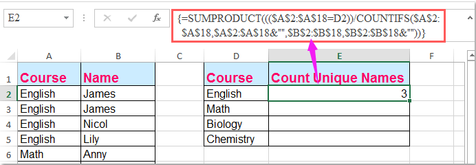
Note: Dalam rumus di atas: A2: A18 adalah data kolom tempat Anda menghitung nilai uniknya, B2: B18 adalah kolom yang ingin Anda hitung nilai uniknya, D2 berisi kriteria yang Anda anggap unik berdasarkan.

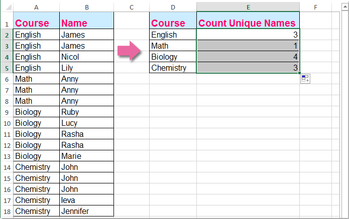
2. Lalu seret gagang isian ke bawah untuk mendapatkan nilai unik dari kriteria yang sesuai. Lihat tangkapan layar:

jumlah doc unik dengan kriteria 3


Artikel terkait:

Bagaimana cara menghitung jumlah nilai unik dalam kisaran di Excel?

Bagaimana cara menghitung nilai unik dalam kolom yang difilter di Excel?

Bagaimana cara menghitung nilai yang sama atau duplikat hanya sekali dalam satu kolom?

Alat Produktivitas Kantor Terbaik

馃 Kutools AI Ajudan: Merevolusi analisis data berdasarkan: Eksekusi Cerdas   |  Hasilkan Kode  |  Buat Rumus Khusus  |  Analisis Data dan Hasilkan Grafik  |  Aktifkan Fungsi Kutools...
Fitur Populer: Temukan, Sorot, atau Identifikasi Duplikat   |  Hapus Baris Kosong   |  Gabungkan Kolom atau Sel tanpa Kehilangan Data   |   Putaran tanpa Formula ...
Pencarian Super: VLookup Beberapa Kriteria    VLookup Nilai Berganda  |   VLookup di Beberapa Lembar   |   Pencarian Fuzzy ....
Daftar Drop-down Lanjutan: Buat Daftar Drop Down dengan Cepat   |  Daftar Drop Down yang Bergantung   |  Multi-pilih Drop Down List ....
Manajer Kolom: Tambahkan Jumlah Kolom Tertentu  |  Pindahkan Kolom  |  Alihkan Status Visibilitas Kolom Tersembunyi  |  Bandingkan Rentang & Kolom ...
Fitur Unggulan: Fokus Kisi   |  Tampilan Desain   |   Bar Formula Besar    Manajer Buku Kerja & Lembar   |  Perpustakaan Sumberdaya (Teks otomatis)   |  Pemetik tanggal   |  Gabungkan Lembar Kerja   |  Enkripsi/Dekripsi Sel    Kirim Email berdasarkan Daftar   |  Filter Super   |   Filter Khusus (filter tebal/miring/coret...) ...
15 Perangkat Teratas12 Teks Tools (Tambahkan Teks, Hapus Karakter, ...)   |   50 + Grafik jenis (Gantt Chart, ...)   |   40+ Praktis Rumus (Hitung usia berdasarkan ulang tahun, ...)   |   19 Insersi Tools (Masukkan Kode QR, Sisipkan Gambar dari Jalur, ...)   |   12 Konversi Tools (Angka ke Kata, Konversi Mata Uang, ...)   |   7 Gabungkan & Pisahkan Tools (Lanjutan Gabungkan Baris, Pisahkan Sel, ...)   |   ... dan banyak lagi

Tingkatkan Keterampilan Excel Anda dengan Kutools for Excel, dan Rasakan Efisiensi yang Belum Pernah Ada Sebelumnya. Kutools for Excel Menawarkan Lebih dari 300 Fitur Lanjutan untuk Meningkatkan Produktivitas dan Menghemat Waktu.  Klik Di Sini untuk Mendapatkan Fitur yang Paling Anda Butuhkan...

Deskripsi Produk


Tab Office Membawa antarmuka Tab ke Office, dan Membuat Pekerjaan Anda Jauh Lebih Mudah

  • Aktifkan pengeditan dan pembacaan tab di Word, Excel, PowerPoint, Publisher, Access, Visio, dan Project.
  • Buka dan buat banyak dokumen di tab baru di jendela yang sama, bukan di jendela baru.
  • Meningkatkan produktivitas Anda sebesar 50%, dan mengurangi ratusan klik mouse untuk Anda setiap hari!
Comments (20)
No ratings yet. Be the first to rate!
This comment was minimized by the moderator on the site
Hi, thanks for this formula, I'm having an issue implementing it across two Worksheets. In my example, your columns A and B are on one sheet, and D and E are on another, which collects similar data from other year-based Sheets. If I put the formula on the sheet where D (Area) and E are, in E it just returns a zero =SUMPRODUCT(((MHST2324[@Team]=[@Area]))/COUNTIFS(MHST2324[@Team],MHST2324[@Team]&"",MHST2324[@School],MHST2324[@School]&"")). However if I put the formula on the Sheet where A (Team) and B (School) are, it works =SUMPRODUCT((([@Team]=Schools[Area]))/COUNTIFS([@Team],[@Team]&"",[@School],[@School]&"")), any ideas as to why?
This comment was minimized by the moderator on the site
Hey, thanks for this formula, I'm having a problem where
This comment was minimized by the moderator on the site
袣谢邪褋褋薪邪褟 褎芯褉屑褍谢邪, 薪芯 泻邪泻 褋写械谢邪褌褜 褔褌芯斜褘 胁 褋褌芯谢斜械褑 A 懈 B 屑芯卸薪芯 斜褘谢芯 锌芯褋褌芯褟薪薪芯 写芯斜邪胁谢褟褌褜 懈 薪械 屑械薪褟褌褜 褎芯褉屑褍谢褍 ? 蟹邪泻褉械锌懈褌褜 薪械 写懈邪锌邪蟹芯薪 邪 褋褌芯谢斜褑褘
This comment was minimized by the moderator on the site
Hello, DM,
In fact, you can enlarg the cell references as you need. For example:
=SUMPRODUCT((($A$2:$A$10000=D2))/COUNTIFS($A$2:$A$10000,$A$2:$A$10000&"",$B$2:$B$10000,$B$2:$B$10000&""))
Please remeber to press Ctrl + Shift + Enter keys together.
Please have a try, hope it can help you!
This comment was minimized by the moderator on the site
Is there a way to do this but not count a blank cell as a value?
This comment was minimized by the moderator on the site
Hello, MB
To count the unqiue values with criteria and skip the blank cell, you should apply the below array formula:
=SUM(--(FREQUENCY(IF($B$2:$B$15<>"",IF($A$2:$A$15=D2,MATCH($B$2:$B$15,$B$2:$B$15,0))),ROW($B$2:$B$15)-ROW(B2)+1)>0))


After pasting the fromula, please press Ctrl + Shift + Enter keys together.

https://www.extendoffice.com/images/stories/comments/comment-skyyang/doc-count-unique-criteria.png

Please try, hope it can help you!
This comment was minimized by the moderator on the site
Thank you very much for this but how does it work with a large data set. I realised it returns #N/A when the data is beyond row 78
This comment was minimized by the moderator on the site
I would need to do something similar but with dates: on a sheet in which the dates are indicated in the first column, many repeated, I would like to know how many different dates there are that meet a certain condition that appears in another column. I am applying that formula but it gives me an error. Could you help me? Thanks.
This comment was minimized by the moderator on the site
Does anyone know what the ampersand-quotes (" &"" ") in the Criteria 1 and 2 portion of the COUNTIFS formula is doing? This formula worked for me I was just hoping to understand it better.
This comment was minimized by the moderator on the site
Worked like a charm. Very much greatful to you.
This comment was minimized by the moderator on the site
OMG.... I have been searching for over a week for a formula that came close to helping me do a distinct count of one column based on another column.... YOURS FINALLY HELPED ;0) I am so happy!!!!!! Now I just need this formula that you posted to do the same thing but based on 2 column instead of one. I am going to try on my own but do you think you can help?
This comment was minimized by the moderator on the site
Hello, EB, To count the unique values based on two columns, please apply the below formula, after entering the formula, please press Ctrl + Shift + Enter keys together to get the correct result.=SUM(IFERROR(($A$2:$A$15=E2)*($B$2:$B$15=F2)/COUNTIFS($C$2:$C$15,$C$2:$C$15,$A$2:$A$15,E2,$B$2:$B$15,F2),0))
Please try, hope it can help you!
This comment was minimized by the moderator on the site
WOAH, you're a savior, thank you for sharing
This comment was minimized by the moderator on the site
Nevermind it did
There are no comments posted here yet
Load More
Please leave your comments in English
Posting as Guest
Rate this post:
0   Characters
Suggested Locations