Loncat ke daftar isi utama

Bagaimana cara mengekstrak nilai unik berdasarkan kriteria di Excel?

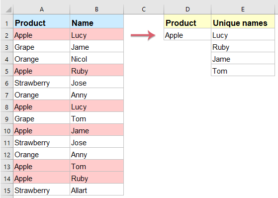
Misalkan, Anda memiliki rentang data kiri yang ingin Anda daftar hanya nama unik kolom B berdasarkan kriteria tertentu dari kolom A untuk mendapatkan hasil seperti gambar di bawah ini. Bagaimana Anda bisa menangani tugas ini di Excel dengan cepat dan mudah?

Ekstrak nilai unik berdasarkan kriteria dengan rumus array

Ekstrak nilai unik berdasarkan beberapa kriteria dengan rumus array

Ekstrak nilai unik dari daftar sel dengan fitur yang berguna


Ekstrak nilai unik berdasarkan kriteria dengan rumus array

Untuk menyelesaikan pekerjaan ini, Anda dapat menerapkan rumus array yang kompleks, lakukan hal berikut:

1. Masukkan rumus di bawah ini ke dalam sel kosong tempat Anda ingin mencantumkan hasil ekstraksi, dalam contoh ini, saya akan meletakkannya ke sel E2, lalu tekan Shift + Ctrl + Masuk kunci untuk mendapatkan nilai unik pertama.

=IFERROR(INDEX($B$2:$B$15, MATCH(0, IF($D$2=$A$2:$A$15, COUNTIF($E$1:$E1, $B$2:$B$15), ""), 0)),"")

2. Kemudian, seret gagang isian ke sel sampai sel kosong ditampilkan, dan sekarang semua nilai unik berdasarkan kriteria tertentu telah terdaftar, lihat tangkapan layar:

Catatan: Dalam rumus di atas: B2: B15 adalah rentang kolom berisi nilai unik yang ingin Anda ekstrak, A2: A15 adalah kolom berisi kriteria Anda berdasarkan, D2 menunjukkan kriteria yang Anda inginkan untuk mencantumkan nilai unik berdasarkan, dan E1 adalah sel di atas rumus yang Anda masukkan.

Ekstrak nilai unik berdasarkan beberapa kriteria dengan rumus array

Jika Anda ingin mengekstrak nilai unik berdasarkan dua kondisi, berikut adalah rumus array lain yang dapat membantu Anda, lakukan seperti ini:

1. Masukkan rumus di bawah ini ke dalam sel kosong di mana Anda ingin mencantumkan nilai unik, dalam contoh ini, saya akan meletakkannya ke sel G2, lalu tekan Shift + Ctrl + Masuk kunci untuk mendapatkan nilai unik pertama.

=IFERROR(INDEX($C$2:$C$15,MATCH(0,COUNTIF(G1:$G$1,$C$2:$C$15)+IF($A$2:$A$15<>$E$2,1,0)+IF($B$2:$B$15<>$F$2,1,0),0)),"")

2. Kemudian, seret gagang isian ke sel sampai sel kosong ditampilkan, dan sekarang semua nilai unik berdasarkan dua kondisi tertentu telah terdaftar, lihat tangkapan layar:

Catatan: Dalam rumus di atas: C2: C15 adalah rentang kolom berisi nilai unik yang ingin Anda ekstrak, A2: A15 dan E2 adalah rentang pertama dengan kriteria yang ingin Anda ekstrak berdasarkan nilai unik, B2: B15 dan F2 adalah rentang kedua dengan kriteria yang ingin Anda ekstrak berdasarkan nilai unik, dan G1 adalah sel di atas rumus yang Anda masukkan.

Ekstrak nilai unik dari daftar sel dengan fitur yang berguna

Terkadang, Anda hanya ingin mengekstrak nilai unik dari daftar sel, di sini, saya akan merekomendasikan alat yang berguna-Kutools untuk Excel, Dengan yang Ekstrak sel dengan nilai unik (termasuk duplikat pertama) utilitas, Anda dapat dengan cepat mengekstrak nilai-nilai unik.

Catatan:Untuk menerapkan ini Ekstrak sel dengan nilai unik (termasuk duplikat pertama), pertama, Anda harus mengunduh Kutools untuk Excel, lalu terapkan fitur dengan cepat dan mudah.

Setelah menginstal Kutools untuk Excel, lakukan seperti ini:

1. Klik sel tempat Anda ingin mengeluarkan hasilnya. (Note: Jangan mengklik sel di baris pertama.)

2. Lalu klik Kutools > Pembantu Formula > Pembantu Formula, lihat tangkapan layar:

3. di Rumus Pembantu kotak dialog, lakukan operasi berikut:

  • Pilih Teks pilihan dari Rumus Tipe daftar drop-down;
  • Lalu pilih Ekstrak sel dengan nilai unik (termasuk duplikat pertama) dari Pilih fromula kotak daftar;
  • Di kanan Masukan argumen bagian, pilih daftar sel yang ingin Anda ekstrak nilai uniknya.

4. Lalu klik Ok tombol, hasil pertama ditampilkan ke dalam sel, lalu pilih sel dan seret pegangan isian ke sel yang ingin Anda daftarkan semua nilai unik sampai sel kosong ditampilkan, lihat tangkapan layar:

Unduh Gratis Kutools untuk Excel Sekarang!


Artikel yang lebih relatif:

  • Hitung Jumlah Nilai Unik Dan Berbeda Dari Sebuah Daftar
  • Misalkan, Anda memiliki daftar panjang nilai dengan beberapa item duplikat, sekarang, Anda ingin menghitung jumlah nilai unik (nilai yang muncul dalam daftar hanya sekali) atau nilai yang berbeda (semua nilai berbeda dalam daftar, artinya unik nilai + nilai duplikat pertama) di kolom seperti gambar kiri yang ditampilkan. Artikel ini, saya akan berbicara tentang cara menangani pekerjaan ini di Excel.
  • Jumlahkan Nilai Unik Berdasarkan Kriteria Di Excel
  • Misalnya, saya memiliki berbagai data yang berisi kolom Nama dan Urutan, sekarang, untuk menjumlahkan hanya nilai unik di kolom Urutan berdasarkan kolom Nama seperti gambar berikut yang ditampilkan. Bagaimana mengatasi tugas ini dengan cepat dan mudah di Excel?
  • Ubah Urutan Sel Dalam Satu Kolom Berdasarkan Nilai Unik Di Kolom Lain
  • Misalkan, Anda memiliki rentang data yang berisi dua kolom, sekarang, Anda ingin mengubah urutan sel dalam satu kolom menjadi baris horizontal berdasarkan nilai unik di kolom lain untuk mendapatkan hasil berikut. Apakah Anda punya ide bagus untuk mengatasi masalah ini di Excel?
  • Gabungkan Nilai Unik Di Excel
  • Jika saya memiliki daftar panjang nilai yang diisi dengan beberapa data duplikat, sekarang, saya hanya ingin menemukan nilai unik dan kemudian menggabungkannya menjadi satu sel. Bagaimana saya bisa mengatasi masalah ini dengan cepat dan mudah di Excel?

Alat Produktivitas Kantor Terbaik

🤖 Kutools AI Ajudan: Merevolusi analisis data berdasarkan: Eksekusi Cerdas   |  Hasilkan Kode  |  Buat Rumus Khusus  |  Analisis Data dan Hasilkan Grafik  |  Aktifkan Fungsi Kutools...
Fitur Populer: Temukan, Sorot, atau Identifikasi Duplikat   |  Hapus Baris Kosong   |  Gabungkan Kolom atau Sel tanpa Kehilangan Data   |   Putaran tanpa Formula ...
Pencarian Super: VLookup Beberapa Kriteria    VLookup Nilai Berganda  |   VLookup di Beberapa Lembar   |   Pencarian Fuzzy ....
Daftar Drop-down Lanjutan: Buat Daftar Drop Down dengan Cepat   |  Daftar Drop Down yang Bergantung   |  Multi-pilih Drop Down List ....
Manajer Kolom: Tambahkan Jumlah Kolom Tertentu  |  Pindahkan Kolom  |  Alihkan Status Visibilitas Kolom Tersembunyi  |  Bandingkan Rentang & Kolom ...
Fitur Unggulan: Fokus Kisi   |  Tampilan Desain   |   Bar Formula Besar    Manajer Buku Kerja & Lembar   |  Perpustakaan Sumberdaya (Teks otomatis)   |  Pemetik tanggal   |  Gabungkan Lembar Kerja   |  Enkripsi/Dekripsi Sel    Kirim Email berdasarkan Daftar   |  Filter Super   |   Filter Khusus (filter tebal/miring/coret...) ...
15 Perangkat Teratas12 Teks Tools (Tambahkan Teks, Hapus Karakter, ...)   |   50 + Grafik jenis (Gantt Chart, ...)   |   40+ Praktis Rumus (Hitung usia berdasarkan ulang tahun, ...)   |   19 Insersi Tools (Masukkan Kode QR, Sisipkan Gambar dari Jalur, ...)   |   12 Konversi Tools (Angka ke Kata, Konversi Mata Uang, ...)   |   7 Gabungkan & Pisahkan Tools (Lanjutan Gabungkan Baris, Pisahkan Sel, ...)   |   ... dan banyak lagi

Tingkatkan Keterampilan Excel Anda dengan Kutools for Excel, dan Rasakan Efisiensi yang Belum Pernah Ada Sebelumnya. Kutools for Excel Menawarkan Lebih dari 300 Fitur Lanjutan untuk Meningkatkan Produktivitas dan Menghemat Waktu.  Klik Di Sini untuk Mendapatkan Fitur yang Paling Anda Butuhkan...

Deskripsi Produk


Tab Office Membawa antarmuka Tab ke Office, dan Membuat Pekerjaan Anda Jauh Lebih Mudah

  • Aktifkan pengeditan dan pembacaan tab di Word, Excel, PowerPoint, Publisher, Access, Visio, dan Project.
  • Buka dan buat banyak dokumen di tab baru di jendela yang sama, bukan di jendela baru.
  • Meningkatkan produktivitas Anda sebesar 50%, dan mengurangi ratusan klik mouse untuk Anda setiap hari!
Comments (40)
No ratings yet. Be the first to rate!
This comment was minimized by the moderator on the site
Thank you so much. This was very very helpful. You Rock!!
This comment was minimized by the moderator on the site
hi everyone..
i have problem..
i got blank result even i press ctrl shift enter together..
This comment was minimized by the moderator on the site
Hi all, Can some help me to get all unique values on one single cell
This comment was minimized by the moderator on the site
Hi, this worked well! Although it takes Excel sooooo long to calculate. Just dragging down 15 cells in a column takes about 15min to calculate... if not longer. Is this normal? If this becomes dynamic it will take a hell of alot of computing time.
This comment was minimized by the moderator on the site
Hello. This is really helpful, however, what If I want a formula that lists the unique values based on multiple criteria. eg. I have a data set which has the following data in a table (after each hyphen is a new column but same row):

Company A - £200 - £100
Company A - £300 - £200
Company B - £300 - £200
Company C - £600 - £200
Company B - £100 - £300
Company D - £0 - £600
Company A - £700 - £100

I want a new data table in a new tab which groups the duplicate values without using an array formula. currently I'm grouping using a pivot table and pasting to my new data table. It's a long process but array formulas make my spreadsheet really slow.

Company A - £1200 - £400
Company B - £400 - £500
Company C - £600 - £200
Company D - £0 - £600

Thanks,
K
This comment was minimized by the moderator on the site
Hello, K,
For solving your problem, I can recommend our useful tool- Kutools for Excel, with its Advanced Combine Rows feature, you can deal with this job quickly. Firstly, you should copy and paste your data into a new worksheet, and then apply htis feature as below screenhsot shown.
You can know more about this feature from: https://www.extendoffice.com/product/kutools-for-excel/excel-combine-duplicate-rows.html
Please download Kutools for Excel and install it, then apply this feature. Full feature free trial 30-day, please try.
This comment was minimized by the moderator on the site
Hi! the formula works really well. I would like to add another criterion, i mean, get the unique answers but using two criteria
This comment was minimized by the moderator on the site
Hi, Giancarlo,
to extract unique values based on multiple criteria, any of the below formula can help you: (after pasting the formula, please press Ctrl + Shift + Enter keys together.)
=IFERROR(INDEX($C$2:$C$11, MATCH(0, COUNTIF(G1:$G$1, $C$2:$C$11)+IF($A$2:$A$11<>$E$2, 1, 0)+IF($B$2:$B$11<>$F$2, 1, 0), 0)), "")
=INDEX($C$2:$C$11, MATCH(0, IF(($A$2:$A$11=$E$2)*($B$2:$B$11=$F$2), COUNTIF($G$1:$G1, $C$2:$C$11), ""), 0))
Please try, hope it can help you!
This comment was minimized by the moderator on the site
Hi. I am using the two conditions formula =IFERROR(INDEX($C$2:$C$11, MATCH(0, COUNTIF(G1:$G$1, $C$2:$C$11)+IF($A$2:$A$11<>$E$2, 1, 0)+IF($B$2:$B$11<>$F$2, 1, 0), 0)), "") to extract a unique list and it works great, but I am struggle to add the SMALL function to get the list sorted as well in ascending order. Are you able to help?
This comment was minimized by the moderator on the site
Is there a way to make this work while ALLOWING for duplicate values? For instance, I want all instances of Lucy to be listed in the results.
This comment was minimized by the moderator on the site
Hello, Konstantin,
To extract all corresponding values including the duplicates based on a specific cell criteria, the following array formula can help you, see screenshot:
=IF(ISERROR(INDEX($A$1:$B$17,SMALL(IF($A$1:$A$17=$D$2,ROW($A$1:$A$17)),ROW(1:1)),2)),"",
INDEX($A$1:$B$17,SMALL(IF($A$1:$A$17=$D$2,ROW($A$1:$A$17)),ROW(1:1)),2))

After inserting the formula, please press Shift + Ctrl + Enter keys together to get the correct result, and then drag the fill handle down to get all values.
Hope this can help you, thank you!
This comment was minimized by the moderator on the site
This has worked great for me with a specific lookup value. However, if I wanted to use a wildcard to look up partial values, how would I do that? For example, if I wanted to lookup all the names associated with KT?

I am using this function to look up cells that contain multiple text. For example if each product also had a sub-product within the same cell but I was only looking for names associated with the sub-product "elf".

KTE - elf
KTE- ball
KTE - piano
KTO - elf
KTO- ball
KTO - piano
This comment was minimized by the moderator on the site
For me the formula does not work. I press ctrl shift enter and i still get an error N/A. I would like to add that i prpared exaclty the same data as in tutorial. What is the reason it does not work?
This comment was minimized by the moderator on the site
How would I get this formula to return each of the duplicates instead of one of each of the names? For instance, in the example above, how would I get the results column (B:B) to return Lucy, Ruby, Anny, Jose, Lucy, Anny, Tom? I'm using this as a budget tool pulling to specific account summaries from a general ledger. However, several of the amounts and transaction descriptions are duplicates in the general ledger. Once the first of the duplicated values is pulled, no more of them get pulled.
This comment was minimized by the moderator on the site
Hi, Joe,
To extract all corresponding values based on a specific cell criteria, the following array formula can help you, see screenshot:
=IF(ISERROR(INDEX($A$1:$B$17,SMALL(IF($A$1:$A$17=$D$2,ROW($A$1:$A$17)),ROW(1:1)),2)),"",
INDEX($A$1:$B$17,SMALL(IF($A$1:$A$17=$D$2,ROW($A$1:$A$17)),ROW(1:1)),2))

After inserting the formula, please press Shift + Ctrl + Enter keys together to get the correct result, and then drag the fill handle down to get all values.
Hope this can help you, thank you!
This comment was minimized by the moderator on the site
Last Question: If I want the results column to return all values not associated with KTE or KTO (so, D:D would be Tom, Nocol, Lily, Angelina, Genna), how would I do that?
This comment was minimized by the moderator on the site
Ok, so it works in the master workbook. There is one exception that I haven't been able to determine the cause of: If the array (in my case, the general ledger that I had beginning in row 3) does not begin in Row 1, the returned values are incorrect. What causes this problem, and which term in the formula fixes it? Thanks again for your help with this!
This comment was minimized by the moderator on the site
So far so good. I'm able to duplicate the results in the test sheet, make changes to the array, and then correct the formula to account for the changes I've made. I plan to move this into the master sheet today and see how it works. Thanks for the help!
There are no comments posted here yet
Load More
Please leave your comments in English
Posting as Guest
×
Rate this post:
0   Characters
Suggested Locations