Bagaimana cara vlookup mengembalikan beberapa nilai dalam satu sel di Excel?
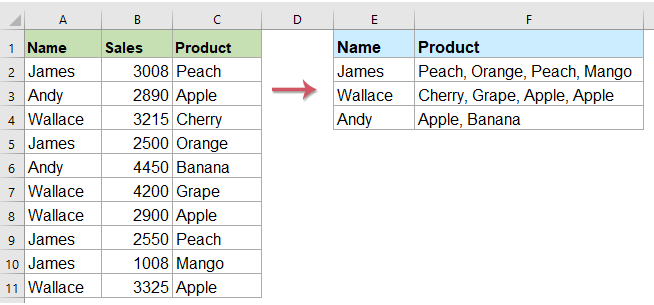
Biasanya, di Excel, saat Anda menggunakan fungsi VLOOKUP, jika ada beberapa nilai yang cocok dengan kriteria, Anda bisa mendapatkan yang pertama. Tapi, terkadang, Anda ingin mengembalikan semua nilai yang sesuai yang memenuhi kriteria ke dalam satu sel seperti gambar berikut yang ditampilkan, bagaimana Anda bisa menyelesaikannya?
- Vlookup untuk mengembalikan semua nilai yang cocok ke dalam satu sel
- Vlookup untuk mengembalikan semua nilai yang cocok tanpa duplikat ke dalam satu sel
Vlookup mengembalikan beberapa nilai ke dalam satu sel dengan User Defined Function
- Vlookup untuk mengembalikan semua nilai yang cocok ke dalam satu sel
- Vlookup untuk mengembalikan semua nilai yang cocok tanpa duplikat ke dalam satu sel
Vlookup untuk mengembalikan beberapa nilai ke dalam satu sel dengan fitur yang berguna
Vlookup untuk mengembalikan beberapa nilai ke dalam satu sel dengan fungsi TEXTJOIN (Excel 2019 dan Office 365)
Jika Anda memiliki versi Excel yang lebih tinggi seperti Excel 2019 dan Office 365, ada fungsi baru - GABUNG TEKS, dengan fungsi canggih ini, Anda dapat dengan cepat melakukan vlookup dan mengembalikan semua nilai yang cocok ke dalam satu sel.
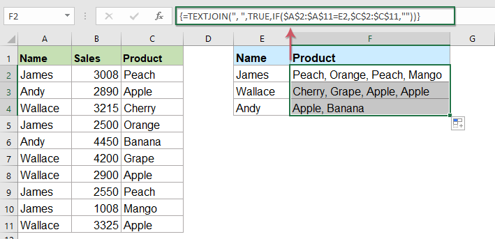
Vlookup untuk mengembalikan semua nilai yang cocok ke dalam satu sel
Harap terapkan rumus di bawah ini ke dalam sel kosong tempat Anda ingin meletakkan hasilnya, lalu tekan Ctrl + Shift + Enter kunci bersama untuk mendapatkan hasil pertama, lalu seret gagang isian ke sel yang ingin Anda gunakan rumus ini, dan Anda akan mendapatkan semua nilai yang sesuai seperti gambar di bawah ini:
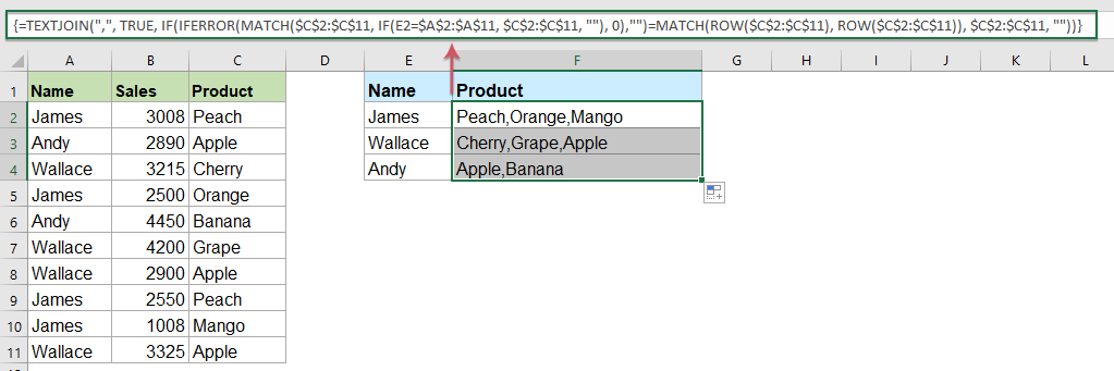
Vlookup untuk mengembalikan semua nilai yang cocok tanpa duplikat ke dalam satu sel
Jika Anda ingin mengembalikan semua nilai yang cocok berdasarkan data pencarian tanpa duplikat, rumus di bawah ini dapat membantu Anda.
Silakan salin dan tempel rumus berikut ke dalam sel kosong, lalu tekan Ctrl + Shift + Enter kunci bersama untuk mendapatkan hasil pertama, dan kemudian salin rumus ini untuk mengisi sel lain, dan Anda akan mendapatkan semua nilai yang sesuai tanpa dulpicate seperti gambar di bawah ini:
Vlookup mengembalikan beberapa nilai ke dalam satu sel dengan User Defined Function
Fungsi TEXTJOIN di atas hanya tersedia untuk Excel 2019 dan Office 365, jika Anda memiliki versi Excel yang lebih rendah, Anda harus menggunakan beberapa kode untuk menyelesaikan tugas ini.
Vlookup untuk mengembalikan semua nilai yang cocok ke dalam satu sel
1. Tahan ALT + F11 kunci, dan itu membuka Microsoft Visual Basic untuk Aplikasi jendela.
2. Klik Menyisipkan > Modul, dan tempel kode berikut di Jendela Modul.
Kode VBA: Vlookup untuk mengembalikan beberapa nilai ke dalam satu sel
Function ConcatenateIf(CriteriaRange As Range, Condition As Variant, ConcatenateRange As Range, Optional Separator As String = ",") As Variant
'Updateby Extendoffice
Dim xResult As String
On Error Resume Next
If CriteriaRange.Count <> ConcatenateRange.Count Then
    ConcatenateIf = CVErr(xlErrRef)
    Exit Function
End If
For i = 1 To CriteriaRange.Count
    If CriteriaRange.Cells(i).Value = Condition Then
        xResult = xResult & Separator & ConcatenateRange.Cells(i).Value
    End If
Next i
If xResult <> "" Then
    xResult = VBA.Mid(xResult, VBA.Len(Separator) + 1)
End If
ConcatenateIf = xResult
Exit Function
End Function
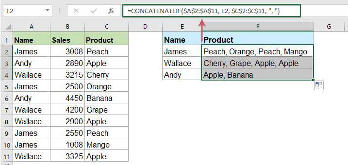
3. Kemudian simpan dan tutup kode ini, kembali ke lembar kerja, dan masukkan rumus ini: =CONCATENATEIF($A$2:$A$11, E2, $C$2:$C$11, ", ") ke dalam sel kosong tertentu di mana Anda ingin menempatkan hasilnya, lalu seret gagang isian ke bawah untuk mendapatkan semua nilai yang sesuai dalam satu sel yang Anda inginkan, lihat tangkapan layar:
Vlookup untuk mengembalikan semua nilai yang cocok tanpa duplikat ke dalam satu sel
Untuk mengabaikan duplikat dalam nilai yang cocok kembali, lakukan dengan kode di bawah ini.
1. Tahan Alt + F11 kunci untuk membuka Microsoft Visual Basic untuk Aplikasi jendela.
2. Klik Menyisipkan > Modul, dan tempel kode berikut di Jendela Modul.
Kode VBA: Vlookup dan mengembalikan beberapa nilai unik yang cocok ke dalam satu sel
Function MultipleLookupNoRept(Lookupvalue As String, LookupRange As Range, ColumnNumber As Integer)
'Updateby Extendoffice
    Dim xDic As New Dictionary
    Dim xRows As Long
    Dim xStr As String
    Dim i As Long
    On Error Resume Next
    xRows = LookupRange.Rows.Count
    For i = 1 To xRows
        If LookupRange.Columns(1).Cells(i).Value = Lookupvalue Then
            xDic.Add LookupRange.Columns(ColumnNumber).Cells(i).Value, ""
        End If
    Next
    xStr = ""
    MultipleLookupNoRept = xStr
    If xDic.Count > 0 Then
        For i = 0 To xDic.Count - 1
            xStr = xStr & xDic.Keys(i) & ","
        Next
        MultipleLookupNoRept = Left(xStr, Len(xStr) - 1)
    End If
End Function
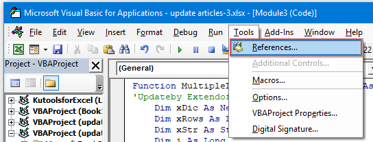
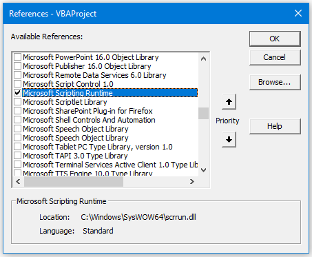
3. Setelah memasukkan kode, selanjutnya klik Tools > Referensi di tempat terbuka Microsoft Visual Basic untuk Aplikasi jendela, dan kemudian, di muncul keluar Referensi - VBAProject kotak dialog, periksa Runtime Microsoft Scripting pilihan dalam Referensi yang Tersedia kotak daftar, lihat tangkapan layar:
 |
 |
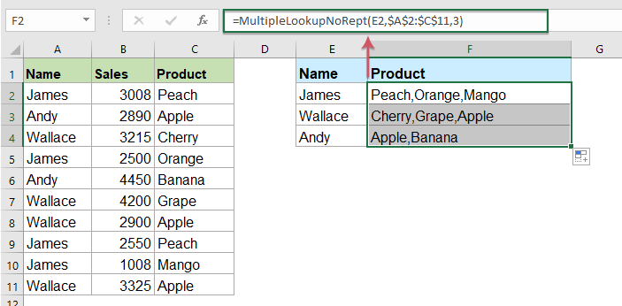
4. Lalu klik OK untuk menutup kotak dialog, simpan dan tutup jendela kode, kembali ke lembar kerja, dan masukkan rumus ini: =MultipleLookupNoRept(E2,$A$2:$C$11,3) into a blank cell where you want to output the result, and then drag the fill hanlde down to get all matching values, see screenshot:
Vlookup untuk mengembalikan beberapa nilai ke dalam satu sel dengan fitur yang berguna
Jika Anda memiliki kami Kutools untuk Excel, Dengan yang Lanjutan Gabungkan Baris fitur, Anda dapat dengan cepat menggabungkan atau menggabungkan baris berdasarkan nilai yang sama dan melakukan beberapa perhitungan yang Anda butuhkan.
Setelah menginstal Kutools untuk Excel, lakukan hal berikut:
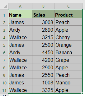
1. Pilih rentang data yang ingin Anda gabungkan satu data kolom berdasarkan kolom lain.
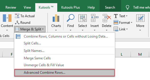
2. Klik Kutools > Gabungkan & Pisahkan > Lanjutan Gabungkan Baris, lihat tangkapan layar:
3. Di muncul keluar Lanjutan Gabungkan Baris kotak dialog:
- Klik nama kolom kunci yang akan digabungkan berdasarkan, lalu klik Kunci utama
- Kemudian klik kolom lain yang ingin Anda gabungkan datanya berdasarkan kolom kunci, dan klik Menggabungkan untuk memilih satu pemisah untuk memisahkan data gabungan.
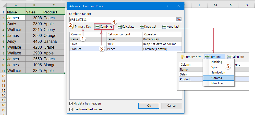
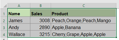
4. Kemudian klik OK tombol, dan Anda akan mendapatkan hasil sebagai berikut:
 |
 |
Unduh dan uji coba gratis Kutools untuk Excel Sekarang!
Artikel yang lebih relatif:
- Fungsi VLOOKUP Dengan Beberapa Contoh Dasar Dan Tingkat Lanjut
- Di Excel, fungsi VLOOKUP adalah fungsi yang andal untuk sebagian besar pengguna Excel, yang digunakan untuk mencari nilai di paling kiri rentang data, dan mengembalikan nilai yang cocok di baris yang sama dari kolom yang Anda tentukan. Tutorial ini membahas tentang cara menggunakan fungsi VLOOKUP dengan beberapa contoh dasar dan lanjutan di Excel.
- Kembalikan beberapa nilai yang cocok berdasarkan satu atau beberapa kriteria
- Biasanya, mencari nilai tertentu dan mengembalikan item yang cocok itu mudah bagi kebanyakan dari kita dengan menggunakan fungsi VLOOKUP. Namun, pernahkah Anda mencoba mengembalikan beberapa nilai yang cocok berdasarkan satu atau lebih kriteria? Pada artikel ini, saya akan memperkenalkan beberapa rumus untuk menyelesaikan tugas kompleks ini di Excel.
- Vlookup Dan Mengembalikan Banyak Nilai Secara Vertikal
- Biasanya, Anda dapat menggunakan fungsi Vlookup untuk mendapatkan nilai pertama yang sesuai, tetapi terkadang Anda ingin mengembalikan semua rekaman yang cocok berdasarkan kriteria tertentu. Artikel ini, saya akan berbicara tentang cara vlookup dan mengembalikan semua nilai yang cocok secara vertikal, horizontal atau ke dalam satu sel.
- Vlookup Dan Kembalikan Beberapa Nilai Dari Daftar Drop Down
- Di Excel, bagaimana Anda bisa vlookup dan mengembalikan beberapa nilai yang sesuai dari daftar turun bawah, yang berarti ketika Anda memilih satu item dari daftar turun bawah, semua nilai relatifnya ditampilkan sekaligus. Artikel ini, saya akan memperkenalkan solusi selangkah demi selangkah.
Alat Produktivitas Kantor Terbaik
Tingkatkan Keterampilan Excel Anda dengan Kutools for Excel, dan Rasakan Efisiensi yang Belum Pernah Ada Sebelumnya. Kutools for Excel Menawarkan Lebih dari 300 Fitur Lanjutan untuk Meningkatkan Produktivitas dan Menghemat Waktu. Klik Di Sini untuk Mendapatkan Fitur yang Paling Anda Butuhkan...
")
Tab Office Membawa antarmuka Tab ke Office, dan Membuat Pekerjaan Anda Jauh Lebih Mudah
- Aktifkan pengeditan dan pembacaan tab di Word, Excel, PowerPoint, Publisher, Access, Visio, dan Project.
- Buka dan buat banyak dokumen di tab baru di jendela yang sama, bukan di jendela baru.
- Meningkatkan produktivitas Anda sebesar 50%, dan mengurangi ratusan klik mouse untuk Anda setiap hari!
")