Loncat ke daftar isi utama

Bagaimana format tanggal bersyarat kurang dari / lebih besar dari hari ini di Excel?

Anda dapat memformat tanggal bersyarat berdasarkan tanggal saat ini di Excel. Misalnya, Anda dapat memformat tanggal sebelum hari ini, atau memformat tanggal yang lebih besar dari hari ini. Dalam tutorial ini, kami akan menunjukkan kepada Anda bagaimana menggunakan fungsi TODAY dalam format bersyarat untuk menyoroti tanggal jatuh tempo atau tanggal yang akan datang di Excel secara detail.

Tanggal format bersyarat sebelum hari ini atau tanggal di masa mendatang di Excel


Tanggal format bersyarat sebelum hari ini atau tanggal di masa mendatang di Excel

Katakanlah Anda memiliki daftar tanggal seperti gambar di bawah ini. Untuk membiarkan tanggal jatuh tempo dan tanggal masa depan terutang, lakukan hal berikut.

1. Pilih rentang A2: A15, lalu klik Format Bersyarat > Kelola Aturan bawah Beranda tab. Lihat tangkapan layar:

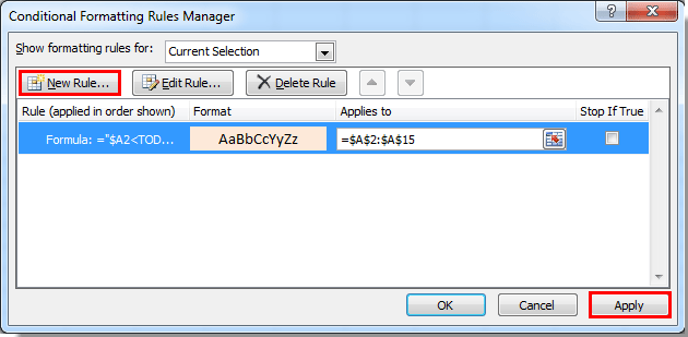
2. Dalam Manajer Aturan Pemformatan Bersyarat kotak dialog, klik Aturan baru .

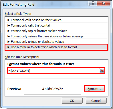
3. Dalam Aturan Pemformatan Baru kotak dialog, Anda perlu:

1). Pilih Gunakan rumus untuk menentukan sel mana yang akan diformat dalam Select a Rule Type bagian;

2). Untuk memformat tanggal yang lebih lama dari hari ini, harap salin dan tempel rumus = $ A2 ke dalam Memformat nilai yang rumus ini benar kotak;

Untuk memformat tanggal masa depan, harap gunakan rumus ini = $ A2> HARI INI ();

3). Klik dibentuk tombol. Lihat tangkapan layar:

4. Dalam Format Cells kotak dialog, tentukan format untuk tanggal jatuh tempo atau tanggal yang akan datang, dan kemudian klik OK .

5. Kemudian kembali ke Manajer Aturan Pemformatan Bersyarat kotak dialog. Dan aturan pemformatan tanggal jatuh tempo dibuat. Jika Anda ingin menerapkan aturan ini sekarang, klik Mendaftar .

6. Namun jika Anda ingin menerapkan aturan tanggal jatuh tempo dan aturan tanggal mendatang secara bersamaan, buat aturan baru dengan rumus format tanggal mendatang dengan mengulangi langkah-langkah di atas dari 2 menjadi 4.

7. Ketika kembali ke Manajer Aturan Pemformatan Bersyarat kotak dialog lagi, Anda dapat melihat dua aturan yang ditampilkan di kotak, klik OK tombol untuk memulai pemformatan.

Kemudian Anda dapat melihat tanggal yang lebih tua dari hari ini dan tanggal yang lebih besar dari hari ini berhasil diformat.

Memformat bersyarat dengan mudah setiap baris n yang dipilih:

Kutools untuk Excel's Shading Baris / Kolom Alternatif utilitas membantu Anda dengan mudah menambahkan pemformatan bersyarat ke setiap baris n dalam pemilihan Excel.
Unduh fitur lengkap jejak gratis 30 hari dari Kutools untuk Excel sekarang!


Artikel terkait:

Alat Produktivitas Kantor Terbaik

馃 Kutools AI Ajudan: Merevolusi analisis data berdasarkan: Eksekusi Cerdas   |  Hasilkan Kode  |  Buat Rumus Khusus  |  Analisis Data dan Hasilkan Grafik  |  Aktifkan Fungsi Kutools...
Fitur Populer: Temukan, Sorot, atau Identifikasi Duplikat   |  Hapus Baris Kosong   |  Gabungkan Kolom atau Sel tanpa Kehilangan Data   |   Putaran tanpa Formula ...
Pencarian Super: VLookup Beberapa Kriteria    VLookup Nilai Berganda  |   VLookup di Beberapa Lembar   |   Pencarian Fuzzy ....
Daftar Drop-down Lanjutan: Buat Daftar Drop Down dengan Cepat   |  Daftar Drop Down yang Bergantung   |  Multi-pilih Drop Down List ....
Manajer Kolom: Tambahkan Jumlah Kolom Tertentu  |  Pindahkan Kolom  |  Alihkan Status Visibilitas Kolom Tersembunyi  |  Bandingkan Rentang & Kolom ...
Fitur Unggulan: Fokus Kisi   |  Tampilan Desain   |   Bar Formula Besar    Manajer Buku Kerja & Lembar   |  Perpustakaan Sumberdaya (Teks otomatis)   |  Pemetik tanggal   |  Gabungkan Lembar Kerja   |  Enkripsi/Dekripsi Sel    Kirim Email berdasarkan Daftar   |  Filter Super   |   Filter Khusus (filter tebal/miring/coret...) ...
15 Perangkat Teratas12 Teks Tools (Tambahkan Teks, Hapus Karakter, ...)   |   50 + Grafik jenis (Gantt Chart, ...)   |   40+ Praktis Rumus (Hitung usia berdasarkan ulang tahun, ...)   |   19 Insersi Tools (Masukkan Kode QR, Sisipkan Gambar dari Jalur, ...)   |   12 Konversi Tools (Angka ke Kata, Konversi Mata Uang, ...)   |   7 Gabungkan & Pisahkan Tools (Lanjutan Gabungkan Baris, Pisahkan Sel, ...)   |   ... dan banyak lagi

Tingkatkan Keterampilan Excel Anda dengan Kutools for Excel, dan Rasakan Efisiensi yang Belum Pernah Ada Sebelumnya. Kutools for Excel Menawarkan Lebih dari 300 Fitur Lanjutan untuk Meningkatkan Produktivitas dan Menghemat Waktu.  Klik Di Sini untuk Mendapatkan Fitur yang Paling Anda Butuhkan...

Deskripsi Produk


Tab Office Membawa antarmuka Tab ke Office, dan Membuat Pekerjaan Anda Jauh Lebih Mudah

  • Aktifkan pengeditan dan pembacaan tab di Word, Excel, PowerPoint, Publisher, Access, Visio, dan Project.
  • Buka dan buat banyak dokumen di tab baru di jendela yang sama, bukan di jendela baru.
  • Meningkatkan produktivitas Anda sebesar 50%, dan mengurangi ratusan klik mouse untuk Anda setiap hari!
Comments (24)
No ratings yet. Be the first to rate!
This comment was minimized by the moderator on the site
I want to highlight a cell if:
1. today's date is greater than the date in another cell or blank (=TODAY()>'APM Tracker'P14) AND ALSO;
2. If the date in P15 is greater than P14 same highlight color AND ALSO;
3. If the date in P15 is less than P14 I do not want the highlight
This comment was minimized by the moderator on the site
Hey All,

I want to get only past due dates in the particular column. Instead of highlighting the cells with color i need the dates to be picked in the column

Any solution for this....
This comment was minimized by the moderator on the site
Alright, I read through this thread and did not see this question asked/answered. I have a column of future dates. I would like to add conditional formatting to flag that date exactly 30 days before (1st color "Hey you should get this done its due in 30 day's") and 7 days ( 2nd color "You procrastinated and now you have 7 days to complete this"). Any help here?
This comment was minimized by the moderator on the site
Hi Michael,
I am not sure I understand your question clearly. If you want to hight the date which is 30 days and 7 days from today. Please use the following formulas to create two formula rules with different highlighted colors:
=D9=TODAY()+30
=D9=TODAY()+7

https://www.extendoffice.com/images/stories/comments/comment-picture-zxm/conditional-formatting.png
If this is not what you need, please attach a screenshot of your data here.
This comment was minimized by the moderator on the site
To ignore cells that have blanks try this:

=AND($A2<>"",$A2<TODAY())

This assumes the cell you have selected is A2 (change this to whatever cell you have currently selected)
To copy this to the applicable cells, change the "Applies to" to the cell range you need.
This comment was minimized by the moderator on the site
Hi Andy Campbell,
Thank you for sharing.
This comment was minimized by the moderator on the site
Hi
I am trying to use condition formatting to allow a cell to be highlighted when an item is past due based on different turn around times (TAT). I have a column with a submitted date which is then used with the #of days from the TAT to automatically give the due date. Using the following formula, =IF(OR(E3="",A3=""),"",DATE(YEAR(A3),MONTH(A3),DAY(A3)+E3))
The condition formatting currently used is "cell value < today()" applies to +$G:$G.
What I would like to do is use the stop if rule to stop the condition formatting if the date entered in column "H" is < or = to todays date.
Thanks Michelle
This comment was minimized by the moderator on the site
if i want highlight the due date with the conditional : today less or equal 30 days from due date
This comment was minimized by the moderator on the site
I am trying to create conditional formatting that will highlight rows older than 14 days in yellow and highlight rows older than 21 days in red. My date column starts in A2, I have the following rules applied, but only yellow is highlighting and just the date column, not the entire row. Can you help? Scott

1. =ISBLANK(A2)=TRUE
2. =A2<TODAY()-14
3. =A2<TODAY()-21
This comment was minimized by the moderator on the site
I want to ignore blank cells which doesn't have a date i.e I do not want blank cells to be highlighted when I am comparing dates<Today(). Please help
This comment was minimized by the moderator on the site
Hi Madhu,
The first method in this artice can help you solve the problem. Please have a try.
https://www.extendoffice.com/documents/excel/2499-excel-conditional-formatting-ignore-blank-zero.html
This comment was minimized by the moderator on the site
1 colum has the dates in it i want another colum to change colour when this formula is applied.

any ideas?
This comment was minimized by the moderator on the site
Hi grant,
Supposing you want to change the cell color in column B based on dates in column A, please select the column B cells (such as B2:B21), and apply the conditional formatting function with the above formulas =$A2>Today() or =$A2<Today().
This comment was minimized by the moderator on the site
Hello! can anyone help me?

I have =TODAY() formula in A1 and need 3 more rules to work as per below

rule 1 all dates 8 to 14 days older than today

rule 2 : all dates older 14 to 30 days than today

rule 3: all dates 31 or more days older than today
This comment was minimized by the moderator on the site
it should be something like this:

if(*cell*+8>Today();if(*cell*+14<Today();"8-14 from today";"N/A"))
There are no comments posted here yet
Load More
Please leave your comments in English
Posting as Guest
Rate this post:
0   Characters
Suggested Locations