Loncat ke daftar isi utama

Bagaimana cara menjumlahkan nilai antara dua tanggal di Excel?

Ketika ada dua daftar di lembar kerja Anda seperti gambar di kanan ditampilkan, satu adalah daftar tanggal, yang lainnya adalah daftar nilai. Dan Anda ingin menjumlahkan nilai antara dua rentang tanggal saja, misalnya, menjumlahkan nilai antara 3/4/2014 dan 5/10/2014, bagaimana Anda bisa menghitungnya dengan cepat? Sekarang, saya perkenalkan rumus untuk meringkasnya di Excel.


Jumlahkan nilai antara dua tanggal dengan rumus di Excel

Untungnya, ada rumus yang bisa meringkas nilai antara dua rentang tanggal di Excel.

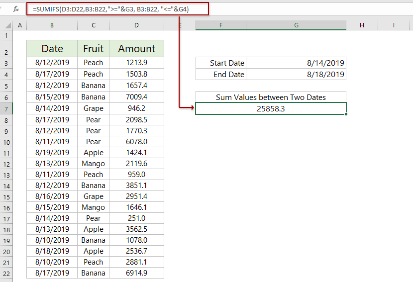
Pilih sel kosong dan ketik rumus di bawah ini, dan tekan Enter tombol. Dan sekarang Anda akan mendapatkan hasil penghitungan. Lihat tangkapan layar:

=SUMIFS(B2:B8,A2:A8,">="&E2,A2:A8,"<="&E3)

Note: Dalam rumus di atas,

  • D3: D22 adalah daftar nilai yang akan Anda simpulkan
  • B3: B22 adalah daftar tanggal yang akan Anda jumlahkan berdasarkan
  • G3 adalah sel dengan tanggal mulai
  • G4 adalah sel dengan tanggal akhir
perhatikan pita Formula terlalu rumit untuk diingat? Simpan rumus sebagai entri Teks Otomatis untuk digunakan kembali hanya dengan satu klik di masa mendatang!
Baca lebih banyak…     Free trial

Menjumlahkan data dengan mudah di setiap tahun fiskal, setiap setengah tahun, atau setiap minggu di Excel

Fitur Pengelompokan Waktu Khusus PivotTable, yang disediakan oleh Kutools for Excel, mampu menambahkan kolom pembantu untuk menghitung tahun fiskal, setengah tahun, nomor minggu, atau hari dalam seminggu berdasarkan kolom tanggal yang ditentukan, dan memudahkan Anda menghitung, menjumlahkan , atau kolom rata-rata berdasarkan hasil yang dihitung dalam Tabel Pivot baru.


Kutools untuk Excel - Tingkatkan Excel dengan lebih dari 300 alat penting. Nikmati uji coba GRATIS 30 hari berfitur lengkap tanpa memerlukan kartu kredit! Get It Now


Jumlahkan nilai antara dua tanggal dengan filter di Excel

Jika Anda perlu menjumlahkan nilai antara dua tanggal, dan rentang tanggal sering berubah, Anda dapat menambahkan filter untuk rentang tertentu, lalu gunakan fungsi SUBTOTAL untuk menjumlahkan antara rentang tanggal yang ditentukan di Excel.

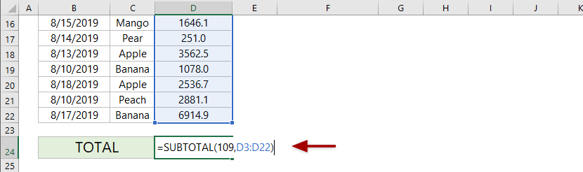
1. Pilih sel kosong, masukkan rumus di bawah ini, dan tekan tombol Enter.

= SUBTOTAL (109, D3: D22)

Catatan: Dalam rumus di atas, 109 berarti jumlah nilai yang difilter, D3: D22 menunjukkan daftar nilai yang akan Anda jumlahkan.

2. Pilih judul rentang, dan tambahkan filter dengan mengklik Data > Filter.

3. Klik ikon filter di tajuk kolom Tanggal, lalu pilih Filter Tanggal > Antara. Dalam dialog Filter Otomatis Kustom, ketikkan tanggal mulai dan tanggal akhir yang Anda perlukan, dan klik OK tombol. Nilai total akan berubah secara otomatis berdasarkan nilai yang difilter.


Artikel terkait:

Alat Produktivitas Kantor Terbaik

🤖 Kutools AI Ajudan: Merevolusi analisis data berdasarkan: Eksekusi Cerdas   |  Hasilkan Kode  |  Buat Rumus Khusus  |  Analisis Data dan Hasilkan Grafik  |  Aktifkan Fungsi Kutools...
Fitur Populer: Temukan, Sorot, atau Identifikasi Duplikat   |  Hapus Baris Kosong   |  Gabungkan Kolom atau Sel tanpa Kehilangan Data   |   Putaran tanpa Formula ...
Pencarian Super: VLookup Beberapa Kriteria    VLookup Nilai Berganda  |   VLookup di Beberapa Lembar   |   Pencarian Fuzzy ....
Daftar Drop-down Lanjutan: Buat Daftar Drop Down dengan Cepat   |  Daftar Drop Down yang Bergantung   |  Multi-pilih Drop Down List ....
Manajer Kolom: Tambahkan Jumlah Kolom Tertentu  |  Pindahkan Kolom  |  Alihkan Status Visibilitas Kolom Tersembunyi  |  Bandingkan Rentang & Kolom ...
Fitur Unggulan: Fokus Kisi   |  Tampilan Desain   |   Bar Formula Besar    Manajer Buku Kerja & Lembar   |  Perpustakaan Sumberdaya (Teks otomatis)   |  Pemetik tanggal   |  Gabungkan Lembar Kerja   |  Enkripsi/Dekripsi Sel    Kirim Email berdasarkan Daftar   |  Filter Super   |   Filter Khusus (filter tebal/miring/coret...) ...
15 Perangkat Teratas12 Teks Tools (Tambahkan Teks, Hapus Karakter, ...)   |   50 + Grafik jenis (Gantt Chart, ...)   |   40+ Praktis Rumus (Hitung usia berdasarkan ulang tahun, ...)   |   19 Insersi Tools (Masukkan Kode QR, Sisipkan Gambar dari Jalur, ...)   |   12 Konversi Tools (Angka ke Kata, Konversi Mata Uang, ...)   |   7 Gabungkan & Pisahkan Tools (Lanjutan Gabungkan Baris, Pisahkan Sel, ...)   |   ... dan banyak lagi

Tingkatkan Keterampilan Excel Anda dengan Kutools for Excel, dan Rasakan Efisiensi yang Belum Pernah Ada Sebelumnya. Kutools for Excel Menawarkan Lebih dari 300 Fitur Lanjutan untuk Meningkatkan Produktivitas dan Menghemat Waktu.  Klik Di Sini untuk Mendapatkan Fitur yang Paling Anda Butuhkan...

Deskripsi Produk


Tab Office Membawa antarmuka Tab ke Office, dan Membuat Pekerjaan Anda Jauh Lebih Mudah

  • Aktifkan pengeditan dan pembacaan tab di Word, Excel, PowerPoint, Publisher, Access, Visio, dan Project.
  • Buka dan buat banyak dokumen di tab baru di jendela yang sama, bukan di jendela baru.
  • Meningkatkan produktivitas Anda sebesar 50%, dan mengurangi ratusan klik mouse untuk Anda setiap hari!
Comments (48)
No ratings yet. Be the first to rate!
This comment was minimized by the moderator on the site
INVOICE DATE TOTAL
01-09-2021 19817
02-09-2021 44791
03-09-2021 26780
03-09-2021 58500
03-09-2021 2029

04-09-2021 79260
04-09-2021 2120
04-09-2021 9187
04-09-2021 5698
04-09-2021 1400
04-09-2021 1900
04-09-2021 7500
04-09-2021 830


i have above data in one sheet and i need date wise total value as below in another sheet,01-09-2021 19817
02-09-2021 44791
03-09-2021 87309
04-09-2021 107895

pls give formula details for itsanjay
This comment was minimized by the moderator on the site
Hi Jett,
You can use the SUMIFS function to sum by multiple criteria simultaneously.
=SUMIFS(sum_range, criteria_range1, criteria1, criteria_range2, criteria2,…, criteria_rangeN, criteriaN)
This comment was minimized by the moderator on the site
What if there are multiple columns to sum up like one for interest, one for penalty, and one for principal amount? and it still need to be between two dates
This comment was minimized by the moderator on the site
hi i have a question related to your topic,if the case is like thisDATE AMOUNT17 SEP 70.000 60.00018 SEP 30.00019 SEP 20.000 10.000IF i use sum if between date 17 sept to 19 sept the 60.000 & 10.000 can't be include in the total.what formulas should i use to include the 60.000 and 10.000 in the total?
This comment was minimized by the moderator on the site
Hi, i have a question related to sumifs:

want to calculate a sum between two dates e.g. start of date and end of date, but at times there are payments which were made in a new month but connected to the expense month, For example if a payment date is Oct 5th but the payment is for September and I would like to show this payment for the month of September, the formula should ignore the Oct 5th date and consider the payment in September. How do i do that
This comment was minimized by the moderator on the site
Help! I can only get this formula to work if I convert to a MM/DD/YYYY format but all of my data is DD/MM/YYYY. The cells are formatted correctly but the formula doesn't work unless I change from eg. 14/01/2020 to 01/14/2020.
This comment was minimized by the moderator on the site
Hi,

can you help me to calculate two working experiences in excel.

Ex: 12 Yeas 3 Months 5 Days - CDB Finance company

9 Years 4 Months 7 Days - Commercial Bank

These are two working experiences in two working places of one person. how to sum these two experiences as a total experience in excel. Please help me.
This comment was minimized by the moderator on the site
Hi Ayesha,
We can suppose the start is 1900/1/0, and add the two date periods to get the end date, and then get the difference between the start date and end date as attached image shown.
Two formulas used:
In Cell B7: =DATE(YEAR(0)+B4+B5,MONTH(0)+C4+C5,DAY(0)+D4+D5)
In Cell B9: =DATEDIF(B1,B7,"Y")&" Years, "&DATEDIF(B1,B7,"YM")&" Months, "&DATEDIF(B1,B7,"MD")&" Days"
This comment was minimized by the moderator on the site
Hi all,

What if one would like to make a date range non-mandatory?

Meaning, let's say that I have two cells with dates in them that are used as my beginning and end date threshold, but when those cells aren't populated, the sum for all dates is pulled from the data set.

My formula (below) has two match criteria with the date ranges at the back of the formula. What I'm trying to do is only filter the sum by the date range if a condition is met (ideally a cell that acts as select Yes or No on "Do you want to limit the sum to a specific date range?"

=SUMIFS(BURN_DATA!$S:$S,BURN_DATA!$R:$R,$A12,BURN_DATA!$H:$H,I$3,BURN_DATA!O:O,">="&I9,BURN_DATA!O:O,"<="&J9)


THANKS IN ADVANCE!
This comment was minimized by the moderator on the site
Aloha, I'm trying to figure out how to sum another column of units, when one column of dates is sequential. Example: I have rows with dates, Mar 1, Mar 2, mar3, then marc 6,7, then march 10.
I need to sum the corresponding units in of another column for mar 1-3, mar 6-7 and mar 10.
This comment was minimized by the moderator on the site
Hi David,
You can use methods introduced in this webpage to sum each period one by one.
Or you can add a helper column before the date column as attached image shown, and then apply the Subtotal feature.
This comment was minimized by the moderator on the site
I am trying to create a holiday calendar to calculate the following information:

Start Date:
End Date (if there is one, otherwise calculate on the entire holiday year_
No of Holidays
Holiday year runs from 01/04 to 31/03 with an entitlement of 20 days plus bank holidays

any help is much appreciated
There are no comments posted here yet
Load More
Please leave your comments in English
Posting as Guest
×
Rate this post:
0   Characters
Suggested Locations