Loncat ke daftar isi utama

Bagaimana menemukan kemunculan n (posisi) karakter dalam string teks di Excel?

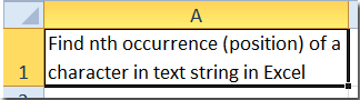
Misalnya ada kalimat panjang di Cell A1, lihat screenshot berikut. Dan sekarang Anda perlu menemukan kemunculan atau posisi ke-3 dari Karakter "c" dari string teks di Sel A1. Tentu saja, Anda dapat menghitung karakter satu per satu, dan mendapatkan hasil posisi yang tepat. Namun, di sini kami akan memperkenalkan beberapa tip mudah untuk menemukan kemunculan atau posisi ke-n karakter tertentu dari string teks dalam sel.


Temukan kemunculan n (posisi) karakter dalam rumus Sel dengan Temukan

Ada dua rumus Find yang dapat membantu Anda menemukan kemunculan atau posisi ke-n karakter tertentu dari string teks dalam sel dengan cepat.

Rumus berikut akan menunjukkan kepada Anda bagaimana menemukan kejadian ke-3 dari "c" di Cell A1.

Temukan Formula 1

Di sel kosong, masukkan rumus = TEMUKAN ("c", A1, TEMUKAN ("c", A1) +2).

doc-find-n-posisi-teks-string2

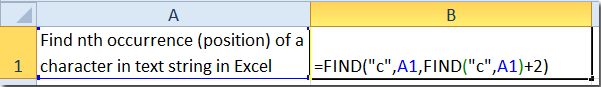
Dan kemudian tekan Enter kunci. Posisi huruf ketiga "c" telah ditampilkan.

Note: Anda dapat mengubah angka 2 di rumus berdasarkan kebutuhan Anda. Misalnya, jika Anda ingin mencari posisi keempat dari "c", Anda dapat mengubah 2 menjadi 3. Dan jika Anda ingin mencari posisi pertama dari "c", Anda harus mengubah 2 menjadi 0.

Temukan rumus 2

Di sel kosong, masukkan rumus = TEMUKAN (CHAR (1), SUBSTITUTE (A1, "c", CHAR (1), 3)), dan tekan Enter kunci.

Note: "3" dalam rumusnya berarti "c" ketiga, Anda dapat mengubahnya berdasarkan kebutuhan Anda.


Hitung kali sebuah kata muncul di sel excel

Jika sebuah kata muncul beberapa kali dalam sel yang perlu dihitung, biasanya, Anda dapat menghitungnya satu per satu. Tetapi jika kata itu muncul ratusan kali, menghitung secara manual merepotkan. Itu Hitung kali sebuah kata muncul fungsi di Kutools untuk Excel's Pembantu Formula grup dapat dengan cepat menghitung berapa kali sebuah kata muncul dalam sel. Uji coba gratis dengan fitur lengkap dalam 30 hari!
 
Kutools for Excel: dengan lebih dari 300 add-in Excel yang praktis, gratis untuk dicoba tanpa batasan dalam 30 hari.

> Temukan kejadian ke-n (posisi) karakter dalam Cell dengan VBA

Sebenarnya, Anda dapat menerapkan makro VB untuk menemukan kejadian atau posisi ke n dari karakter tertentu dalam satu sel dengan mudah.

Langkah 1: Tahan ALT + F11 kunci, dan itu membuka Microsoft Visual Basic untuk Aplikasi jendela.

Langkah 2: Klik Menyisipkan > Modul, dan tempelkan makro berikut di Jendela Modul.

VBA: Temukan posisi ke-n karakter.

Function FindN(sFindWhat As String, _
sInputString As String, N As Integer) As Integer
Dim J As Integer
Application.Volatile
FindN = 0
For J = 1 To N
FindN = InStr(FindN + 1, sInputString, sFindWhat)
If FindN = 0 Then Exit For
Next
End Function

Langkah 3: Sekarang jika Anda ingin menemukan kemunculan yang tepat dari posisi "c" ketiga di sel A1, masukkan rumus = FindN ("c", A1,3), dan tekan tombol Enter kunci. Kemudian itu akan mengembalikan posisi yang tepat di sel tertentu sekaligus.


Temukan kejadian ke-n (posisi) karakter di Sel dengan Kutools for Excel

Jika Anda tidak menyukai formula dan VBA, Anda dapat mencoba alat praktis - Kutools untuk Excel, Dengan yang Rumus grup, Anda dapat menemukan utilitas - Temukan kemunculan n karakter untuk mengembalikan posisi ke-n karakter dalam sel dengan cepat.

Kutools untuk Excel, dengan lebih dari 300 fungsi praktis, membuat pekerjaan Anda lebih mudah. 

Setelah pemasangan gratis Kutools for Excel, lakukan seperti di bawah ini:

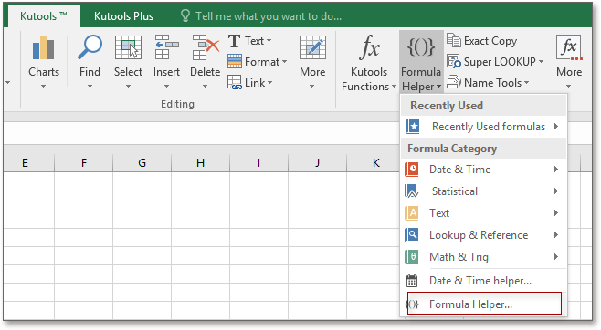
1. Pilih sel yang ingin Anda kembalikan hasilnya dan klik Kutools > Pembantu Formula > Pembantu Formula . Lihat tangkapan layar:

2. Kemudian di popping Pembantu Formula dialog, lakukan seperti di bawah ini:

1) Pilih Lookup dari daftar drop-down Jenis Formula bagian;

2) Pilih Temukan di mana karakter muncul ke-N dalam sebuah string in Pilih rumus bagian;

3) Pilih sel yang berisi string yang Anda gunakan, lalu ketik karakter yang ditentukan dan kejadian n ke dalam kotak teks di Masukan argumen bagian.

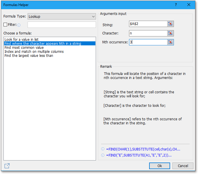
3. klik Ok. Dan Anda mendapatkan posisi kejadian n dari karakter dalam sebuah string.


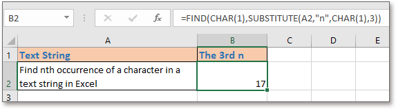
Alat Produktivitas Kantor Terbaik

🤖 Kutools AI Ajudan: Merevolusi analisis data berdasarkan: Eksekusi Cerdas   |  Hasilkan Kode  |  Buat Rumus Khusus  |  Analisis Data dan Hasilkan Grafik  |  Aktifkan Fungsi Kutools...
Fitur Populer: Temukan, Sorot, atau Identifikasi Duplikat   |  Hapus Baris Kosong   |  Gabungkan Kolom atau Sel tanpa Kehilangan Data   |   Putaran tanpa Formula ...
Pencarian Super: VLookup Beberapa Kriteria    VLookup Nilai Berganda  |   VLookup di Beberapa Lembar   |   Pencarian Fuzzy ....
Daftar Drop-down Lanjutan: Buat Daftar Drop Down dengan Cepat   |  Daftar Drop Down yang Bergantung   |  Multi-pilih Drop Down List ....
Manajer Kolom: Tambahkan Jumlah Kolom Tertentu  |  Pindahkan Kolom  |  Alihkan Status Visibilitas Kolom Tersembunyi  |  Bandingkan Rentang & Kolom ...
Fitur Unggulan: Fokus Kisi   |  Tampilan Desain   |   Bar Formula Besar    Manajer Buku Kerja & Lembar   |  Perpustakaan Sumberdaya (Teks otomatis)   |  Pemetik tanggal   |  Gabungkan Lembar Kerja   |  Enkripsi/Dekripsi Sel    Kirim Email berdasarkan Daftar   |  Filter Super   |   Filter Khusus (filter tebal/miring/coret...) ...
15 Perangkat Teratas12 Teks Tools (Tambahkan Teks, Hapus Karakter, ...)   |   50 + Grafik jenis (Gantt Chart, ...)   |   40+ Praktis Rumus (Hitung usia berdasarkan ulang tahun, ...)   |   19 Insersi Tools (Masukkan Kode QR, Sisipkan Gambar dari Jalur, ...)   |   12 Konversi Tools (Angka ke Kata, Konversi Mata Uang, ...)   |   7 Gabungkan & Pisahkan Tools (Lanjutan Gabungkan Baris, Pisahkan Sel, ...)   |   ... dan banyak lagi

Tingkatkan Keterampilan Excel Anda dengan Kutools for Excel, dan Rasakan Efisiensi yang Belum Pernah Ada Sebelumnya. Kutools for Excel Menawarkan Lebih dari 300 Fitur Lanjutan untuk Meningkatkan Produktivitas dan Menghemat Waktu.  Klik Di Sini untuk Mendapatkan Fitur yang Paling Anda Butuhkan...

Deskripsi Produk


Tab Office Membawa antarmuka Tab ke Office, dan Membuat Pekerjaan Anda Jauh Lebih Mudah

  • Aktifkan pengeditan dan pembacaan tab di Word, Excel, PowerPoint, Publisher, Access, Visio, dan Project.
  • Buka dan buat banyak dokumen di tab baru di jendela yang sama, bukan di jendela baru.
  • Meningkatkan produktivitas Anda sebesar 50%, dan mengurangi ratusan klik mouse untuk Anda setiap hari!


Comments (28)
No ratings yet. Be the first to rate!
This comment was minimized by the moderator on the site
Your formula to find the Nth occurrence of a character in a string does not work. Using your example, adding 2 to the results of the imbedded find ensures a starting position for the initial find of a position beyond the 1st two c's but changing the +2 to +3 does not yield the position of the 4th "c", it simply starts the search one character deeper into the string and the result is still the 3rd "c". To find the 4th "c" the search must begin beyond the position of the 3rd "c". I look forward to your new solution.
This comment was minimized by the moderator on the site
Hello, David

Yes, as you said, the first formula does not work correctly, you can apply the second formula:
=FIND(CHAR(1),SUBSTITUTE(A2,"c",CHAR(1),2))

Note: The number "2" in the formula means the second "c", if you want to get the third, fourth "c", just change the number 2 to 3,4 as you need.
Please try, hope it can help you!
This comment was minimized by the moderator on the site
Find formula1 is imperfect. It will be a great help if it is removed. I have lost lot of time trying for 4th occurance of "a" in "vedanarayanan" Thanks.
This comment was minimized by the moderator on the site
To handle the exception of the formula, you can use same with if and iserro
=IF(ISERR(FIND("c",A1,FIND("c",A1)+2)),FIND("c",A1,FIND("c",A1)+0),FIND("c",A1,FIND("c",A1)+2))
This comment was minimized by the moderator on the site
"Substitute" lets you find the Nth occurrence of a term, so combine it with "find" as follows (where 5=5th occurrence):

=FIND(CHAR(1),SUBSTITUTE(A1,"c",CHAR(1),5))
This comment was minimized by the moderator on the site
Excellent! I am glad I scrolled up to review other comments after posting my own.
This comment was minimized by the moderator on the site
This is the correct answer! please replace this whole article with this one line of code.....
This comment was minimized by the moderator on the site
The first formula is completely useless and wrong but it works just correct for this example as the first and second "c"s are adjacent. The correct formula is:


For 2nd occurence -
=FIND("c",A1,FIND("c",A1)+1)

For 3rd occurence -
=FIND("c",A1,FIND("c",A1,FIND("c",A1)+1)+1) and so on...
This comment was minimized by the moderator on the site
Absolutely agree. The +2, or +3 etc.....entirely depends on the spacing between the n and (n+1) occurences of "c". Thus you would have to manually adjust for every cell if you were trying to copy this formula down a column for instance. Essentially the same as manually counting.


Ex. Let's try to find the 4th occurrence of "c" in cell A1 using the provided formula. Per the article we should use +3 in our nested FIND function to find the 4th occurrence.


Text in Cell A1:

"cab car abc cole cube"

Manually counting, the 4th occurrence is the "c" in cole in the character position of 13.


=FIND("c",A1,FIND("c",A1)+3)

The nested function, FIND("c",A1) will find the first occurrence of "c" in position 1.

Therefore,

FIND("c",A1)+3 = 1+3 = 4

Plugging that back into our formula,

=FIND("c",A1,FIND("c",A1)+3) = FIND("c",A1,1+3) = FIND("c",A1,4)

This new formula will look for the first occurrence of "c" beginning from character position 4. The 4th character in the string is the space just after cab.

Therefore, the formula will find the "c" in car and return the value of 5 for our formula. As we know from manually counting we are looking for 13 as the output.
This comment was minimized by the moderator on the site
The firs formula works correct in my version, in the note, it has explained how to find the third or forth or nth "c".

Note: You can change the 2 in the formula based on your needs. For example, if you want to find the fourth position of "c", you can change the 2 to 3. And if you want to find the first position of "c", you shuold change 2 to 0.
This comment was minimized by the moderator on the site
Try to find out the position of the second c with the first sentence of my above comment as the string using the first formula. You'll get to know how correct it is!
This comment was minimized by the moderator on the site
Hello all,

I have a text in an Excel cell " BY TRANSFER-NEFT*HDFC0000001*N08745987123546*J0032331*KUMAR--"

I need a function to extract just "N08745987123546"

Thanks
This comment was minimized by the moderator on the site
Hello, do you want to extract the numbers after No and the number of numbers are fixed? If so, you can use Kutools for Exccel's Extract text function, type No????to extract.
This comment was minimized by the moderator on the site
HI ALL,
I have a text in an Excel cell " BY TRANSFER-NEFT*HDHC0065431*N053112345624801*K0038331*krishna--"
I need a function to extract just "N053112345624801"
This comment was minimized by the moderator on the site
Formula 1 doesn't work on fourth, fifth, sixth etc. so (+3,4,5) will always show third position of letter "c" which is 19 second formula is working though.
This comment was minimized by the moderator on the site
Hello all, I have a text in an Excel cell "23 floyd lane, longville,KN 14564" I need a function to extract just "longville" Thanks
This comment was minimized by the moderator on the site
If you must use a function, try: =TRIM(MID(A1,SEARCH(",",A1)+1,SEARCH("!@#",SUBSTITUTE(A1,",","!@#",2))-SEARCH(",",A1)-1)) Otherwise, you might consider Data > Text to Columns > Delimited (using a comma as the separator).
This comment was minimized by the moderator on the site
Try this: =INDEX(SMALL(IF(MID(A1,MATCH(ROW(INDIRECT(1&":"&LEN(A1))),ROW(INDIRECT(1&":"&LEN(A1))),0),1)="c",MATCH(ROW(INDIRECT(1&":"&LEN(A1))),ROW(INDIRECT(1&":"&LEN(A1))),0),""),MATCH(ROW(INDIRECT(1&":"&LEN(A1)-LEN(SUBSTITUTE(A1,"c","")))),ROW(INDIRECT(1&":"&LEN(A1)-LEN(SUBSTITUTE(A1,"c","")))),0)),2) where "c" is the character required and 2 is the position. Note this is an array formula.
This comment was minimized by the moderator on the site
this is simpler: =INDEX(SMALL(IF(MID(A1,ROW(INDIRECT(1&":"&LEN(A1))),1)="c",ROW(INDIRECT(1&":"&LEN(A1))),""),ROW(INDIRECT(1&":"&LEN(A1)-LEN(SUBSTITUTE(A1,"c",""))))),2)
There are no comments posted here yet
Load More
Please leave your comments in English
Posting as Guest
×
Rate this post:
0   Characters
Suggested Locations